December 3, 2007

REVISITING RENDERING STRATEGIES AND OPTIONS

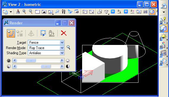
1. THE FENCE TOOL

1.1 Use the Fence tool to optimize rendering tests. Ensure that the render tool "target" is set to fence.

1.2 When rendering for the entire view window, ensure that the render tool "target" is reset to "view".

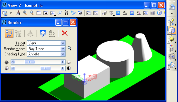
Note that the ACS triad will not appear in images rendered out to file through the untilties/image/save dialog process.

2. BUMP MAPPING

2.1 Use bump mapping to suggest the appearance of materials at a more abstract level, sometimes more effective than more explicit  texture maps used towards the same purpose.

bump map	texture map

2.1 Bump maps can also be created inventively in photoshop towards the description of materials that need some varied surface relief patterns such as water. Ensure that the size of the bump map is mapped to master units. Use the raytrace rendering tool for these examples.

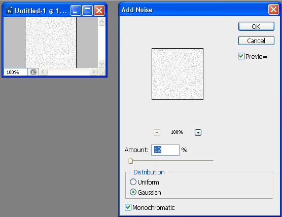
Here, a 100 x 100 pixel image created in Photoshop is filtered with a Gausian noise pattern. In Photoshop, create a 100 x 100 pixel image, and then go to filer/noise/add noise too. The image below demonstrates the use  the Gausian monocrhomatic option. The image is then saved to a "jpg" file format.

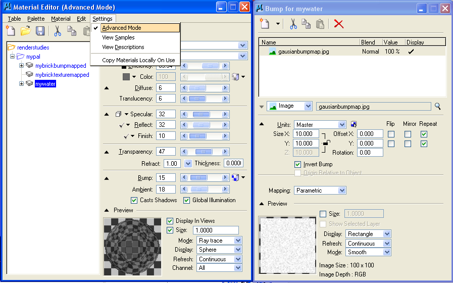
Load the bump map jpg image into the definition of a new material in Microstation and size it to a master unit or multiple of a master unit. Go to "Advanced Model" in the Material Editor.  In the editor, turn on transparency and reflection, reduce the "value" of the color, and begin to adjust other attributes to the lighting conditions and as may be fitting in the particular model. In the dialog boxes below, the bump map is sized to 10 x 10 master units and set to a low intensity value of 15. The ambient light quality is also low. The color is dark gray. Diffuse light levels are low as is translucency. The specular and reflectivitive parameters are set to 32, but the finish value is lower at 10. Transparency is set to 47 on a scale of 1 to 100.

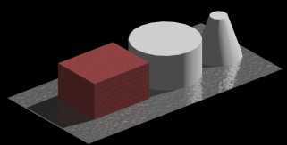
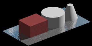
The resulting rendering lacks the reflection of sky and so it is relatively less convincing  in appearance.

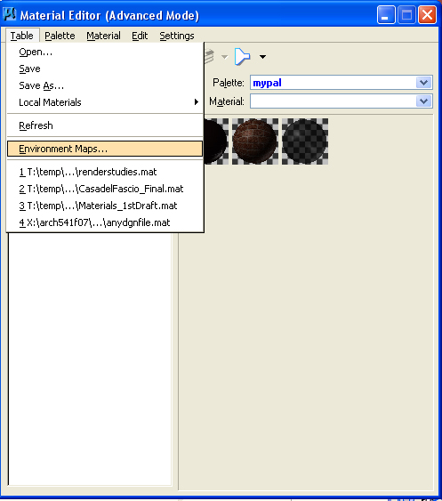
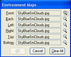
However, when adding an environmental map for a sky, the reflection off the water seems more convincing. That is, in the Material Editor, open the environment dialog map tool and then load an image (e.g., "SkyBlueSmClouds.jpg" to be reflected by the water ).

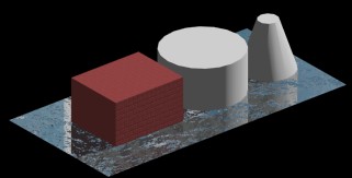
Within the raytracing settings, turn off the "visible environment" option. This ensures that the environmental images are just seen as reflections and not directly. The resulting image is as follows:

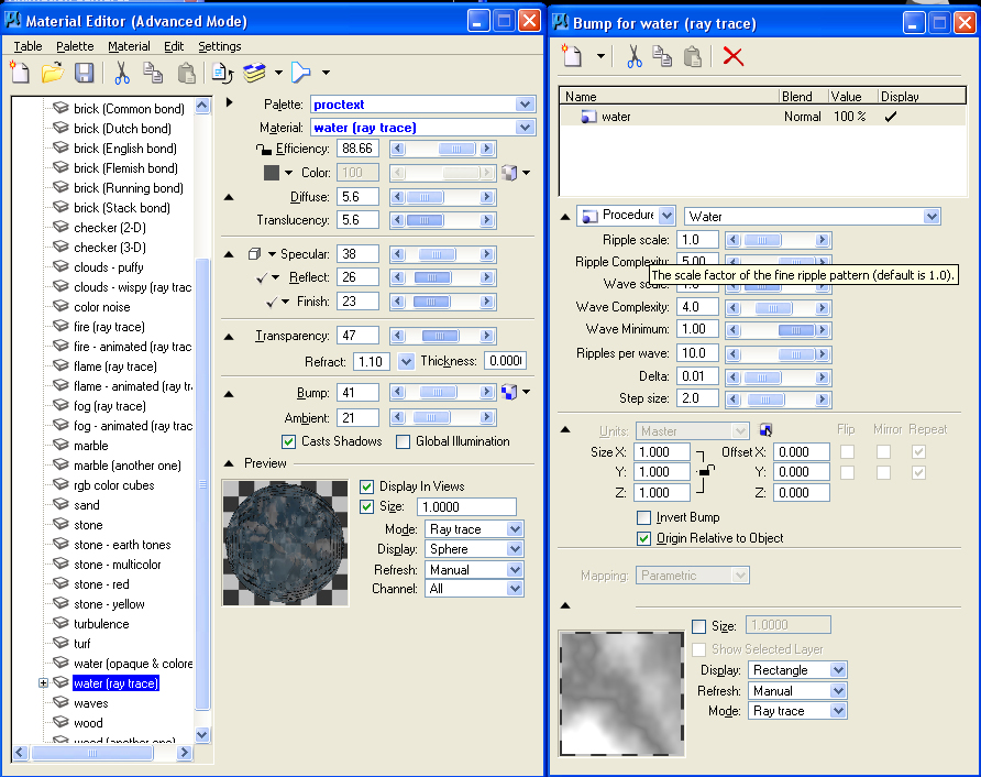
Procedurally based descriptions of water can also provide a more nuanced rendering. Within the "proctext" file, there's a standard procedure file for water that can be used without the environmental sky maps referred to in the previous example. The parameters have been set below to facilitate water in the model. Letting the mouse hover over a parameter of the "proctext" material reveals its purpose, as in the image at right below.

This results in the following rendering.

3. TRANSPARENCY MAPS

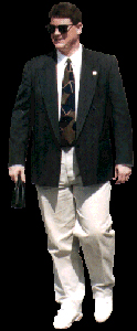
Any photograph of a person, plan or other object can be used as the basis for a transparency map. Here, you paint out the color surrounding the object in "black" or some other uniform color. The file needs to be saved as a true 24 bit color file("tif" rather than "jpg") so that the transparency of the surrounding color is clean. The following image should be saved as a "tif"  file as the beginning point in defining such a transparency mapped material.

More such people images are posted in the classes folder under:

G:\Arch541-Mark-F07\Examples\people\transparencymaps

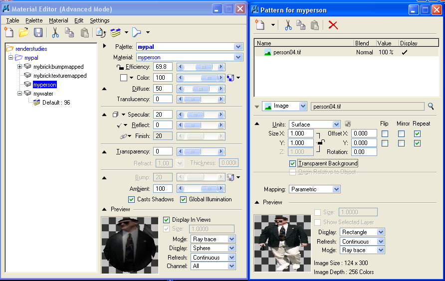
The dialog box for defining such a material as a texture map would appear as indicated in the next image. Note that the source  image file is stretched to the full scale of any surface and not set to master units. Thus the dimensions of the surface it is applied to  detemines the scale of the man in this figure.

The material assigned to the yellow rectangle would then appears as indicated below.

before material assignment	after material assignment

4. RPC FILES

RPC files are provided by commercial retailers who will occasionally provide samples. These files will reorient to the view desired. Commercial sites for obtaining such figures are: http://3dpopulate.com and http://www.archvision.com/. The use of such figures requires the Microstation plugin available through the visualization menu, the last sub-palette and icon indicated below in the dialog box used to select an RPC file and place it. These files can consist of a number of images or frames that provide varied views syncronized with each new view orientation towards the model.

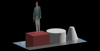
Note that two renderings from different camera positions capture the RPC figure in 3D. However, the first figure of the man developed through transparency mapping appears paper-thin when viewed from some angles. For example, compare the first and second figures below.

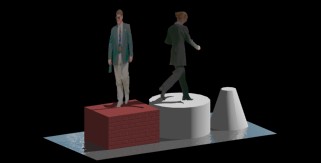juxtaposition of transparency map with rpc figure	juxtaposition of transparency map with rpc figure

See a few free samples of RPC files at

G:\Arch541-Mark-F07\Examples\people\simplerpcfiles

5. 3D WHAREHOUSE

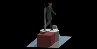
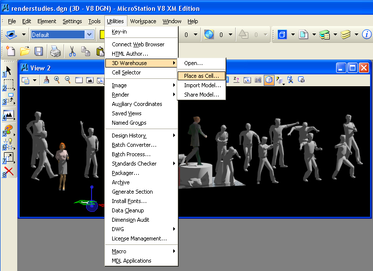
Microstation's implementation of 3D Wharehouse allows direct insertion of 2D and 3D  figures(saved  in the sketchup format) into a 3D model. The dialog box under the utilties menu goes to a web search engine for grabbing 3D and 2D human figures as well as other objects. Some of the 3D objects  may add substantial rendering time to a model, but have the advantage of being  more easily adapted to different views of the model. Note, the option selected under 3D Wharehouse should be "Place as Cell". The 3D Wharehouse links to web site that provides many different downloadable 3D models. The example below was provided by searching under "people" and then choosing "Assorted People 3D" authored by "Distressed American.

6. DISTANCE CUE

Distance cueing is a simple low-computer time cost solution to giving the appearance of diffuse lighting to a 3D model. We setup the appropriate options under the Settings/Rendering/Setup dialog box. Beginning with the General Tab, we set the fog color to light blue in the dialog box depicted below. Then in the View Tab, we set the distance cue to fog  for a specific view (e.g., view4).

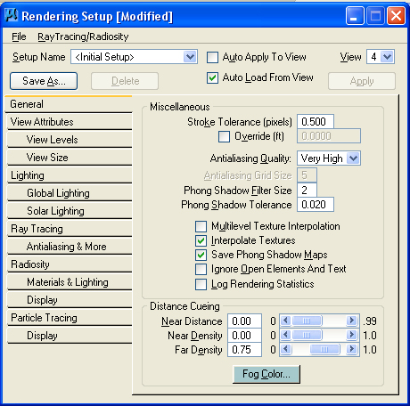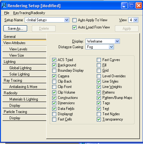general tab	view specific tab

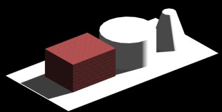
Using also background map for view 4 (see workshop 7 notes), we can see a difference where the  activation of the distance cue occurs in the right image below.

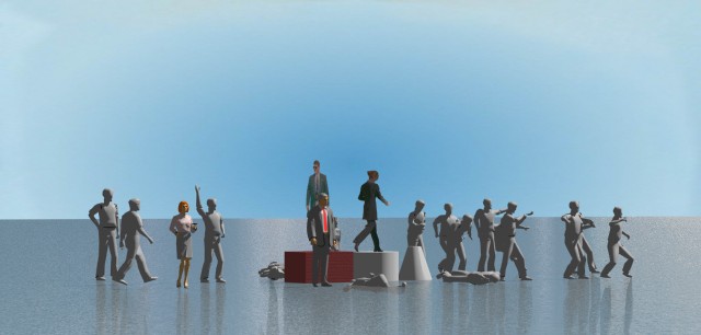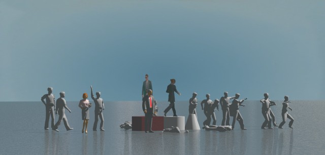before distance cue	after distance cue