CAAD: GENERATIVE COMPONENTS & PROCESS BASED DESCRIPTION

PART I: Generative Components (GC)
An Associative Geometrical Modeling Tool with Constraints

General Background

GC is an associative geometrical modeling tool that uses constraints. Geometry can be associative in the sense that the transformation of one element will be intentionally linked to the transformation of other elements. A constraint is a designed restriction on how elements may be transformed or in some specific way determines how objects may be tied together.

For a simple example, a door may be associative with an opening in a wall. The resizing of a door may be automatically linked to the resizing of the opening in a wall. The opening of a door may also have constraints with respect to the hinges which connect the door to the wall and restrict how it may move. More abstract associations between geometrical elements leads to geometrical models that are more easily changed to fit emerging directions in a design project. This first introduction of GC will demonstrate the concepts needed to construct a twisting tower. Next week, we will look at more advanced approach, where we rely more upon scripting as a way to build geometry.

Specifics of Generative Components

The building blocks of a generative components model are referred to as  features. Examples of features include a point, a line, an ellipse, an arc, a bspline, a surface, a polygon mesh. Points constitute one of the most basic feature types. Other types of features are defined in terms of points. For example, a line feature may be defined by two point features (end points).

Example: Line determined by two points.

A directed graph describes the dependency relationship that exists between geometrical elements. For example the coordinate system is the basis for the definition of two points, and, in turn, the points are the basis for the definition of a line. Within most CAD systems, these dependency relationships are somewhat hidden from the end user. Within Generative Components these dependency relationships are more explicitly developed by and exposed to the user. Thus, the user can more self-evidently move any one of the points and so as to more directly redefine the line.

Directed symbolic graph of elements.

Similarly, points can determine a bspline curve. In turn, bspline curves can determine surfaces. And, surfaces can determine the components of a paneling system. These directed relationships are defined such that changing the points can in turn propagate changes to the bsplines, and in turn, the bsplines propagate changes to the surfaces, and, again in turn, the surfaces propagate changes to the paneling systems. By exposing all the elements of this dependency hierarchy, it is easier to make dynamic changes to a computer model.

Transaction File Window

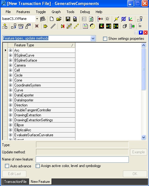
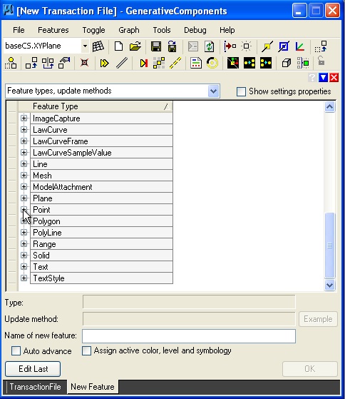
Generative Components is a "transaction based" modeling method. The transactions used to create geometry, rather than the geometry itself, is stored in a "gct" generative components transaction file such as "mydesign.gct". The transaction file manger window is the basic Graphical User Interface to controlling and managing the transactions. The window contains definintions for a number of feature types that may used to construct a geometrical model, such as Arc, BSplineCurve, BSplineSurface, etc., as indicated below.

Simple Example for Point on Line

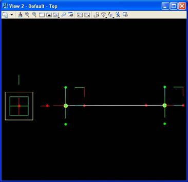
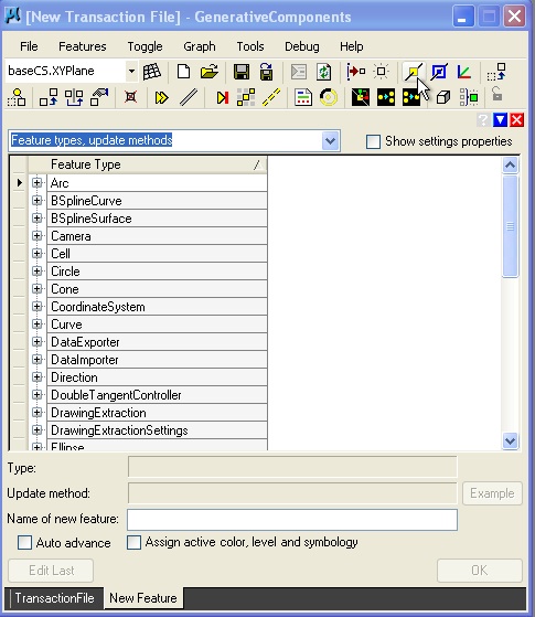
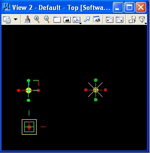
The description of a line simpleline.gct begins with placing points directly in View 2, using a short-cut to the point feature from the icons located at the top of the transaction file manager. The place point icon is located at the arrow cursor in the image below (a yellow square with a diagonal line).

The point is placed by using the left-mouse button and placing the cursor at the desired location in View 2.

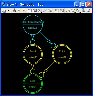
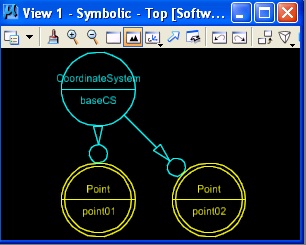
In a separate graphical window, a symbolic directed graph indicates that the two points have been created relative to the "baseCS" coordinate system.

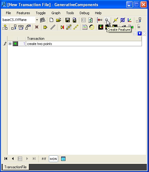
Selecting the "transaction file" tab at the lower left-hand corner of the transaction manager dialog window, and then selecting the green recorder icon, the placement of the two points can be recorded as a single transaction.

Select transaction file tab and hit record button.	Tranaction is listed and description "create two points" is added by user.

To add the line, we select the "create feature" icon. The result is that the feature types are once again listed. We now can select the "line" feature".

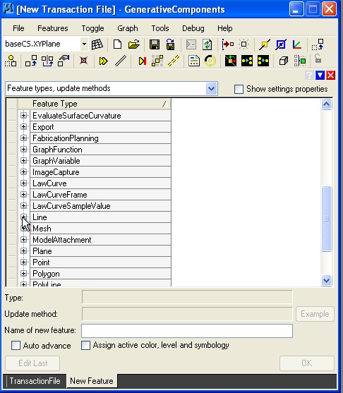Select the create feature button.	Select the line feature.

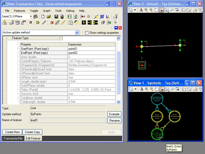
Opening the line feature provides for a number of "update methods" from which the "ByPoints" update method is selected.

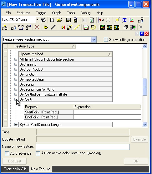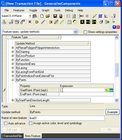Select ByPoints update methods.	Place cursor in StartPoint text box.

Holding the control key down in turn for each textbox "StartPoint and "EndPoint" and moving the cursor into the view 2 window, each of the two points is selected.

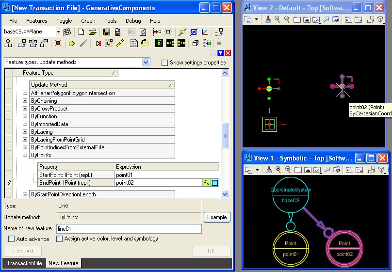
Selection of the "OK" button in the lower right hand corner of the tranaction file manager initiates the final step to creating the line.

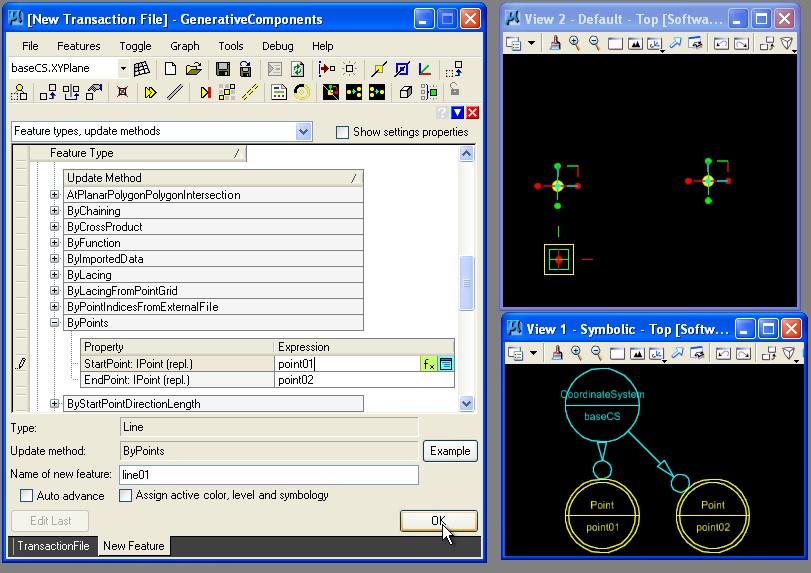
Once created the line is reflected in the symbolic graph.

As before, we can now record the line as a transaction, by selecting the "TransactionFile" tab and hitting the record button.

Select transaction file tab and hit record button.	Tranaction is listed and description "add line to transaction" is added by user.

In the final step, the "create feature" button is used one more time to select a "point" feature. The "ByParameterAlongCurve" update method is selected. The user identifies the "Curve" by holding down the control key and placing the mouse of the line, and also enters a value of 0.45 to establish a parameter for the point along the line.

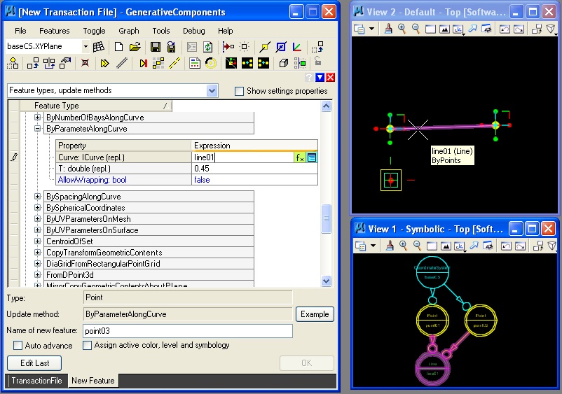Select Point feature.	Enter line01 in ByParameterAlongCurve update method.

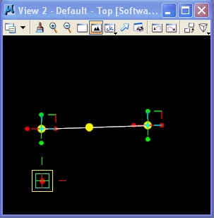
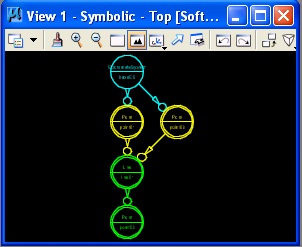
The last step results in a Point feature 45% along the distance of the line from point01 to point02, and also an expansion to the symbolic graph.

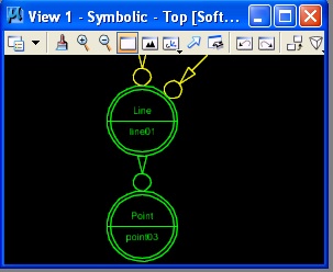Point added to line.	Symbolic graph expanded.	Zoom widow to directed graph line01 -> point03

The resulting transaction is now recorded and the entire transaction file can be save via the "File/Save dialog box".

Variables

Variables can be used to store values in memory that are the basis for describing geometrical elements and their numerically ordered relationships.

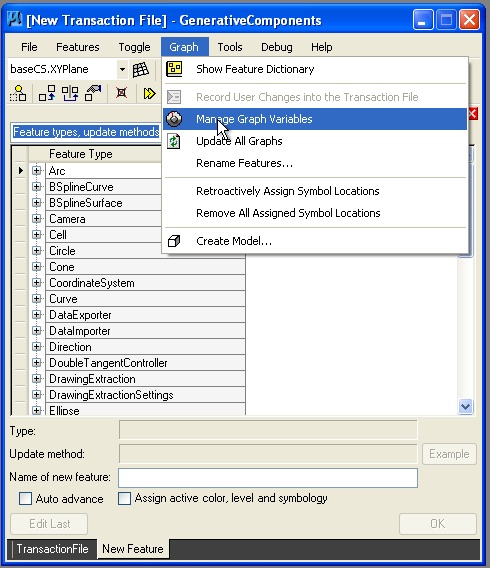
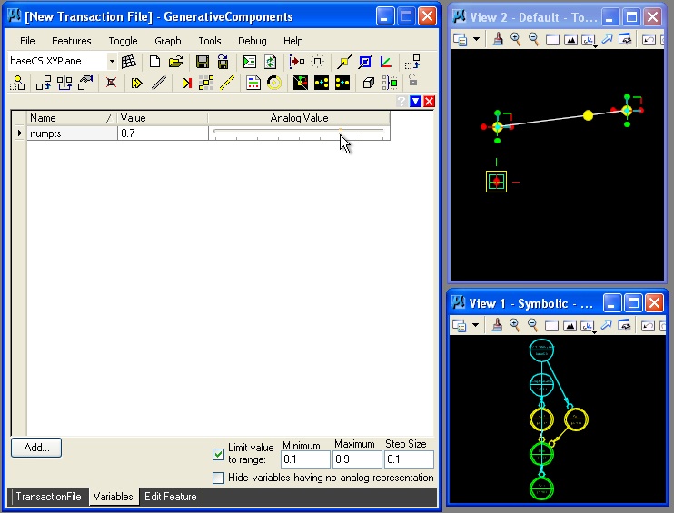
Remaking the previous example as a new file ptonline.gct, we could create a variable "numpts" to hold a numerical value for the position of the point on the line between the two end points point01 and point02. If "numpts = 0.5", then then the position of the point would be 0.5 on a scale of 0 to 1 of the distance from point02 to point02. Typically, we would setup the variable as the first transaction in the program by going to the menu item "Graph -> Variables".

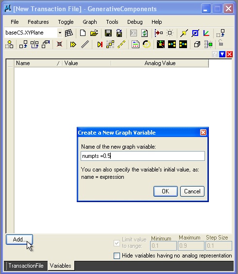
In the dialog box that follows, we iniatiate the value of "numpts" to 5.0, and we also setup a range of values from 0.1 to 1.9 in increments of 0.1. Thus, the variable "numpts" may take on the values of 0.1, 0.2, 0.3, 0.4, 0.5, 0.6, 0.7, 0.8, and 0.9.

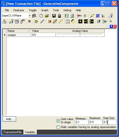Initiate value of numpts at 5.0	Establish a range of values from 0.1 to 0.9 by increments of 0.1

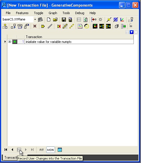
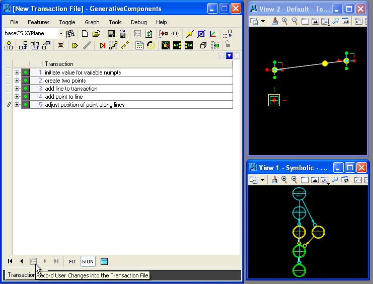
By selecting the "TransactionFile Tab", we may record this first transaction as "initiate value of variable for numpts".

As in the case of previos example, we now add a two points and a line. However, when we arrive at the step to add point parametrically along the line, we use the variable "numpts" rather than a specific numerical value, as shown in the image below.

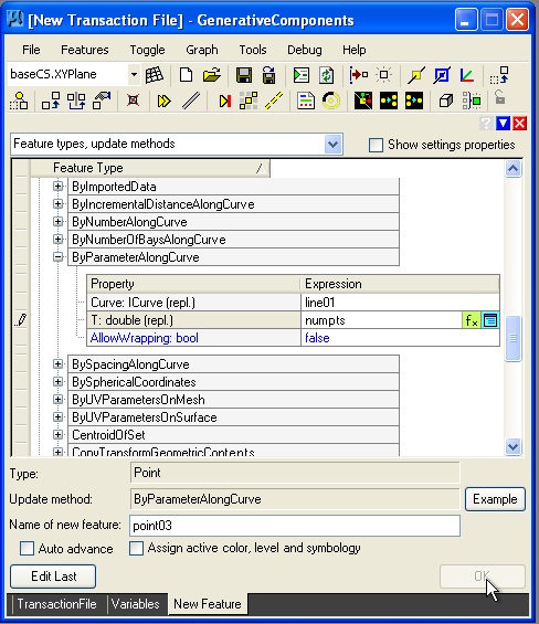
Now, we have a point on the line in a position controlled by the variable "numpts".

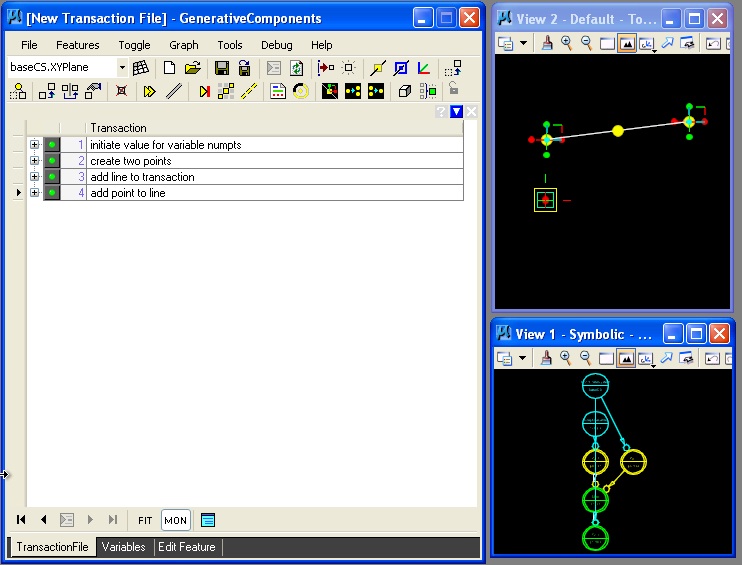
Given the setup of the variable, we can go back to the menu item "Graph -> Variables" and adjust the value of "numpts" and cause the point on the line to move from left to right.

This last transaction may also be saved as a part of the "TransactionFile"

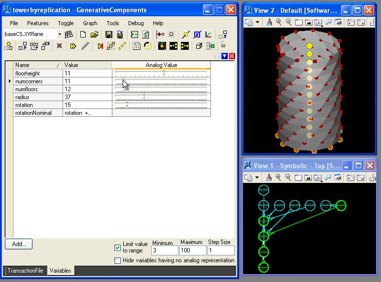
Similarly,  in the example below, variables were used in a more elaborate way to create variations a twisting tower towerbyreplication.gct:

Example Twisting Tower Created with the Use of Variables

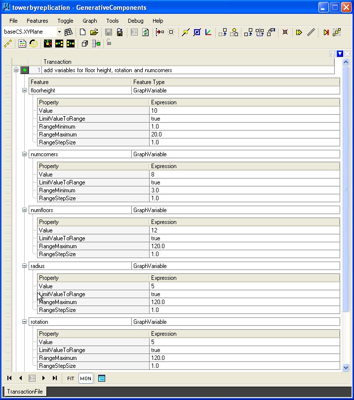
Within GC, variables are referred to as features, similar to points, lines, and other geometrical elements. For describing a tower the following variables might be used

floorheight = ceiling height of each floor
numfloors = number of floors in the tower
numcorners = number of corner pts on the tower
radius = total radius of tower
rotation = floor to floor rotation of twisting tower

These variables may be defined with predetermined minimum, maximum and step values in some cases. Step values determine the minimal change in value for a variable that is possible. For example, the number of floors may change by the step value “1”, such that a 10 floor building, may step in value from 10 to 11 or 10 to 9 or some other increment of 1.

Within GC, these variables would be developed in the following dialog box:

Series and Geometry

The Series (1,5,1) refers to a sequence of numbers that begins with the number 1, concludes with the number 5, and that is incremented by the step size of 1. That is, the Series (1,5,1) is the set of numbers 1, 2, 3, 4, 5. More generally, the series notation system is specified in terms of (start value, max value, step size value). Similarly, the Series (0, numfloors * floorheight, floorheight) uses variables to insert the numerical values.  Combing a series with the variables noted in the table of values above, the Series {0, numfloors * floorheight, floorheight} would be equivalent to (0, 100, 10), or the set of numbers 0, 10, 20, 30, 40, 50, 60, 70, 80, 90, 100, 110 and 120. Series are used to determine a set of ponts in the example of a tower below.

Update Methods Involving the Use of Series

For geometrical features such as points, lines, arcs, etc., there are a variety of update methods that may be used to initiate features as well as update the description of them.   In the dialog box below, a point feature is defined in terms a Series expression incorporated into the  “ByCylindricalCoordinates” update method.

Within the dialog box above, a cylindrical point array could have been defined more simply with the use of constant numerical values.  In particular the point “point01” could have been described in terms of 1) the coordinate system of reference "baseCS" , 2) its radius distance "1"master units (feet)  from the origin of the coordinate system, 3) an angular rotation of "45" from the x-axis of the coordinate system, and 4) and a height of "0" master units along the z-axis of the coordinate system. That is, a point may be defined as:

That is, the point sits 45 degrees rotated counter-clockwise from the x-axis of the base coordinate system at the distance of 1 master unit and elevation 10 master units along the z-axis.

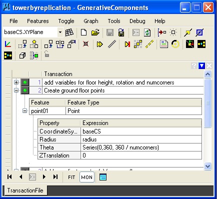
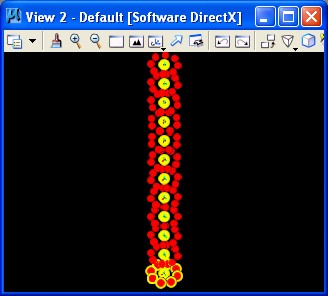
In the approach actually used, taking adantage of a Series, we might define a cylindrical array of points through the use of variables:

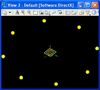
Given that numcorners = 8, The expression "Theta = Series (0, 360, 360/ numcorners)" establishes the series of points at rotation valuues of 0, 45, 90, 135, 180, 225, 270, 315, and 360 degrees, thus generating 9 points in the array depicted in the figure above at the height of z = 0;.

Continuing with a further use of a series, we might also express the Ztranslation as a series:

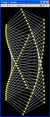
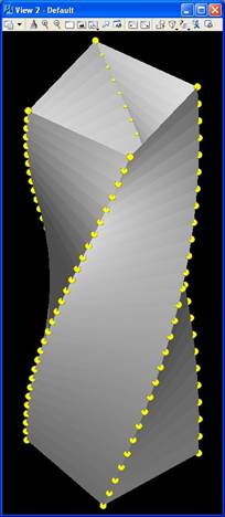
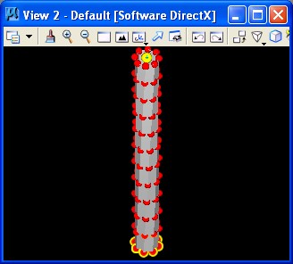
With additional features and transactions as described in the towerbyreplication.gct file, we would get a tower with variable controls yeilding the following image:

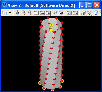The construction of the tower proceeds in six basic steps:

1. Create the variables.

2. Determine the corner points through a cylindrical array

3. Create a set coordinate systems stacked on top of each other.

4. Copy the base points to the new coordinate systems.

5. Replicate the corner points (a technique use to realize the inference of a set of geometrical entities)

6. Add polygonal surfaces to the points.

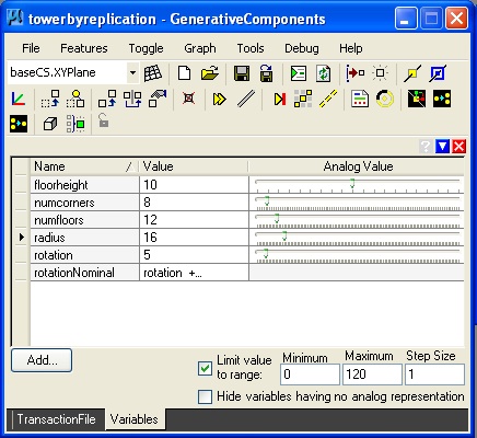
With the variables established for control, the "graph -> manage graph variables" dialog box is opened and adjustments made to variables "floorheight", "numcorners", "numfloors", and "radius" in the situation captured below.

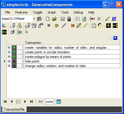
Examples

1. Simple Circle simplecircle.gct

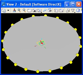Key feature(s):

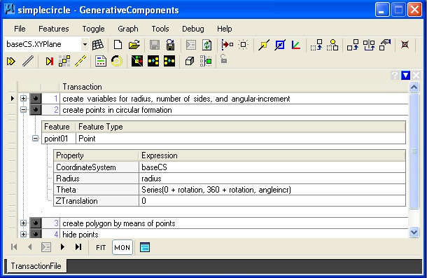
In this example, the point01 is established as a Series based upon a variable for "angleincr" from the origin. Thus if the" angleincr" is 45, then the resulting number of points is 9 at the following degree values: 0, 45, 90, 135, 180, 215, 260, 315, 360.

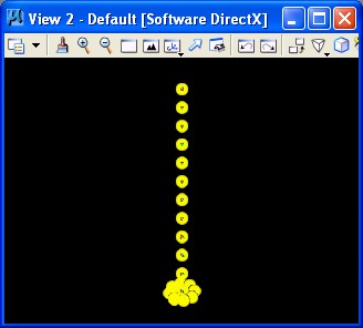
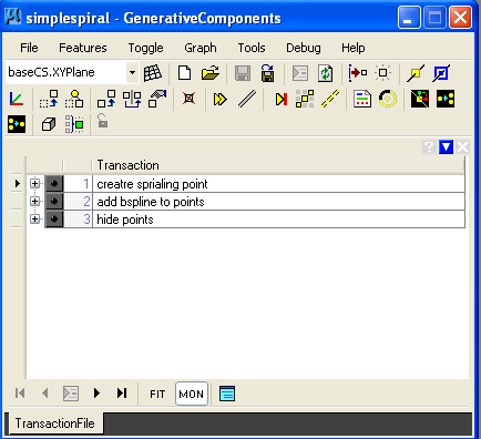
2. Simple Spiral simplespiral.gct

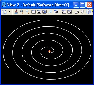Key feature(s):

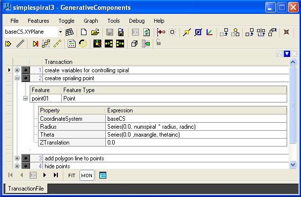
In this example, the radius expands outward and the angular increment of each successive point spins around the origin.

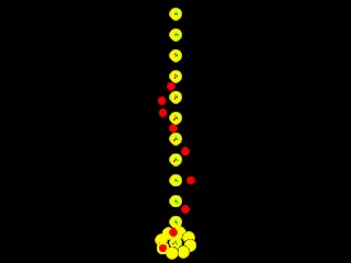
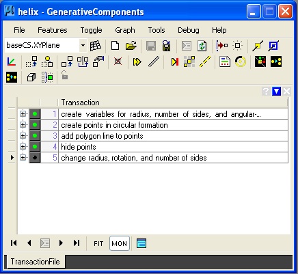
3. Helix helix.gct

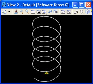Key feature(s):

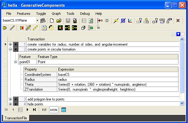
The helix is distinguished from the spiral by adding a series for Ztranslation.

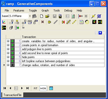
4. Ramp ramp.gct

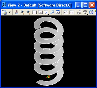Key feature(s):

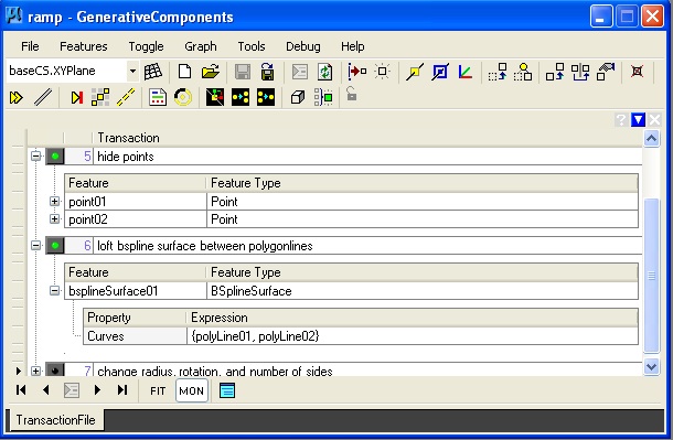
The ramp consists of two sprirals (two helix curves), and a bsplinesurface is then lofted between them.

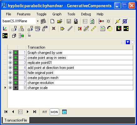
5. Hyperbolic Parabolic Surface hyperbolicpar.gct

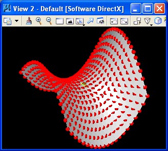Key feature(s):

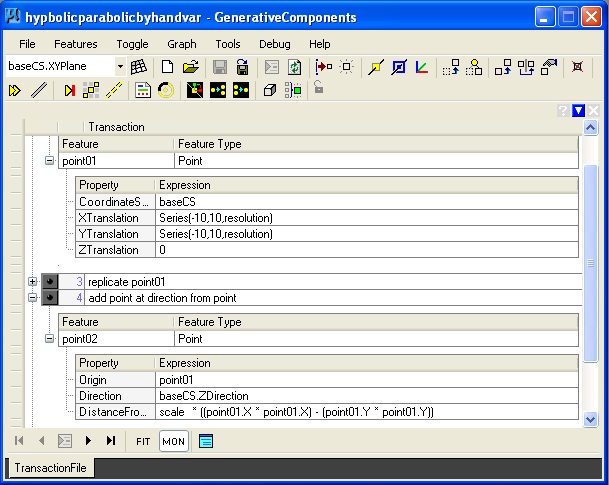
The hyperbolic parabolic surface is based on establising a series of points along the ground plane (step 2 above), replication of the series of points to establish a base grid of points along the grounds plane, and then determining a point at the height of scalar * (x * x) - (y * y) for each point on the ground plane.

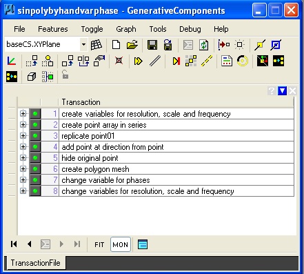
6. Sine Polygon sinpoly.gct

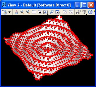Key feature(s):

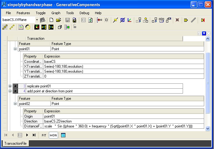
The method of building a Sine surface is similar to that of building a hyperbolic parabolic surface. The script begins by establising a series of points along the ground plane (step 2 above), replication of the series of points to establish a base grid of points along the grounds plane (step 3), and then determining a point at the height of Sine function applied to the distance of each point from the origin. scalar * sin (sqrt ((x * x) + (y * y))) for each point on the ground plane. The variable phase is used to vary the position of the Sine surface relative to the origin. The variable frequency is used to multiply the number of times the Sine curve appears at distances of 360 units form the origin.