COMPUTER AIDED
ARCHITECTURAL DESIGN
Workshop 10 Notes,
Week of November 9, 2009
Editing by
Projection,
Fence Tools, Cutting Solids with Surfaces, GC Examples with Functions
PART
I: FENCE TOOLS
Fence tools allow
you to select a
portion of a view window and to perform
operations on it, such as editing,
deleting, moving, copying, rotating, scaling or stretching geometrical
elements. You can also render a sub-portion of a window
through
the use of a fence tools. The fence tool is projected into
the
view window to perform these various operations.
1. COPY AND CLIP OPERATION
Within
MIcrostation V8i,
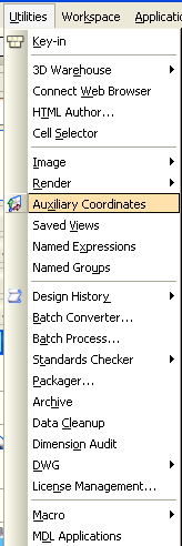
start a new drawing, open the
Utilities>Auxiliary Coordinates dialog box. Use
the save ACS icon
in upper left-hand
corner and save the current default ACS plane as "base".
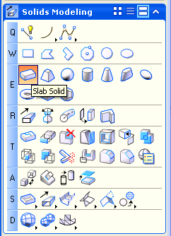
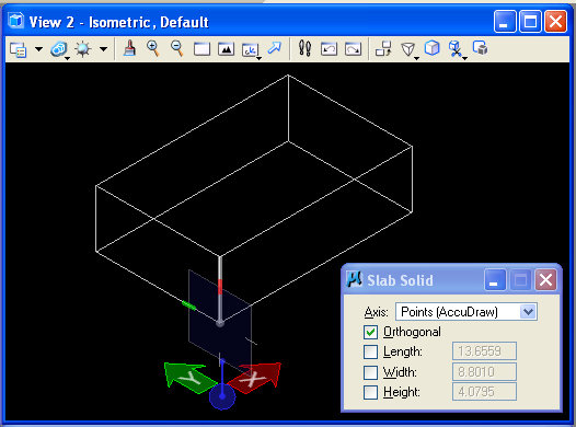
Turn on the ACS PLane lock by opening the padlock symbol at the lower part of the screen. Next, use the Solids Modeling, "Slab Solid" tool
to create a solid slab on the
ground plane.
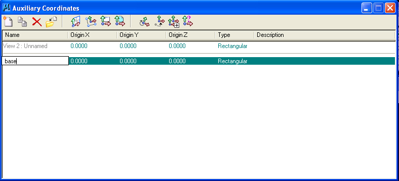
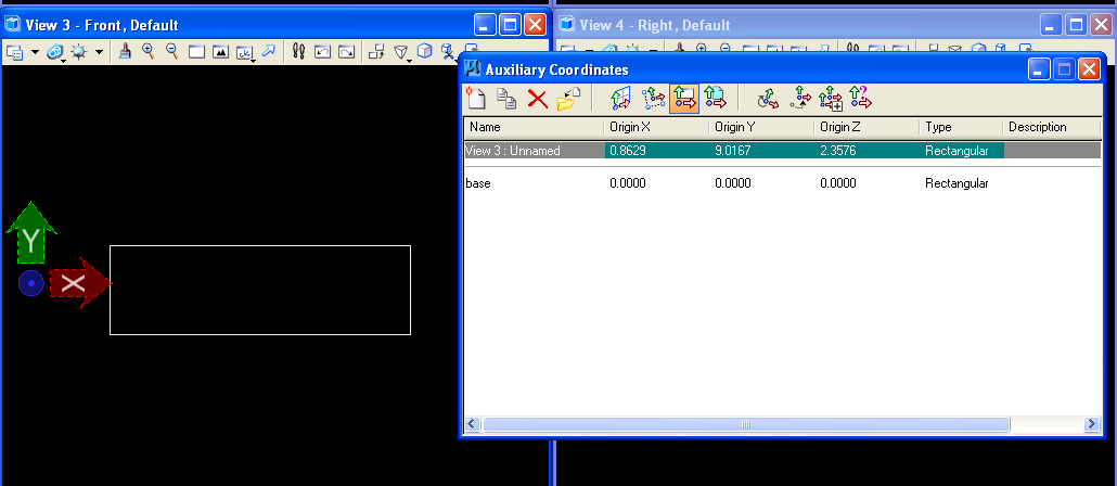
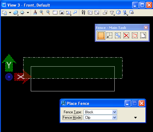
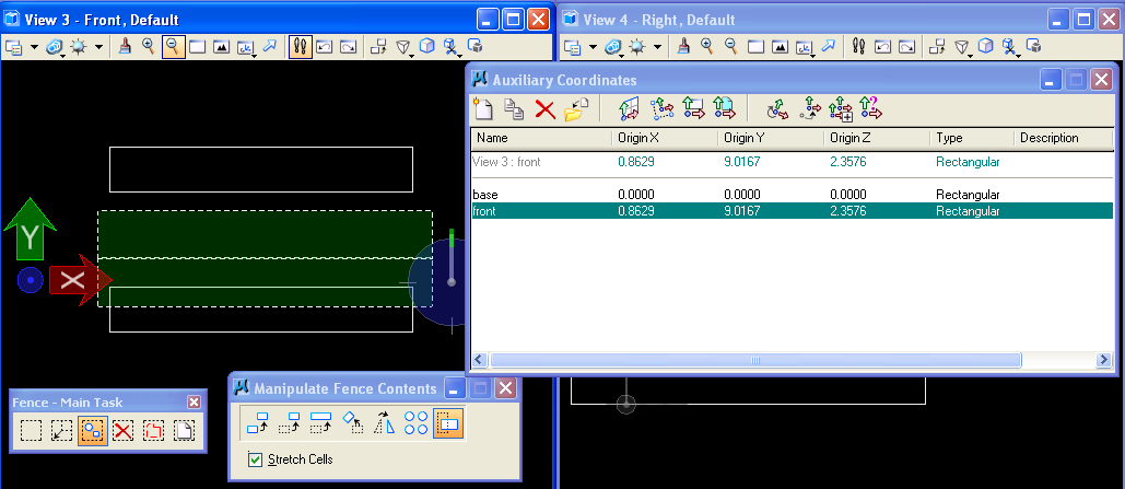
Select the front view (View 3) and use the "Define auxiliary
coordinates by view" icon , highlighted in the Auxiliary
Coordinates
dialog box below (7th icon from left-hand side), to create an ACS in
the
front view window.
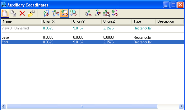
Save the new ACS as "front" within the Auxiliary Coordinates
dialog box.
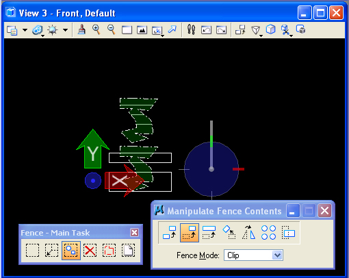
Open the fence tools subpalette from the main task menu (#2 key).
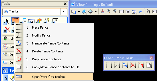
Draw
a
"Fence" in the front view window with "Fence Mode" set to
"Clip". This mode
isolates what's inside the fence from the outside.
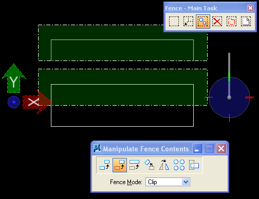
Select the "Manipulate Fence
Contents Icon" (second icon in the Fence palette) andnthe "Move"
option, and enter two data points in the front view with to
clip off and move upward
the geometry that is encompassed within the fence.
This is a
quick boolean operation. Here we are working from a 2D projection of
the fence onto the objects from the view plane.
Similarly, select the top view
window. Select the "base" ACS form
the
Auxiliary Coordinates Dialog box, and repeat the same move
operation on the upper "Y" axis portion of the cubes from the top view.
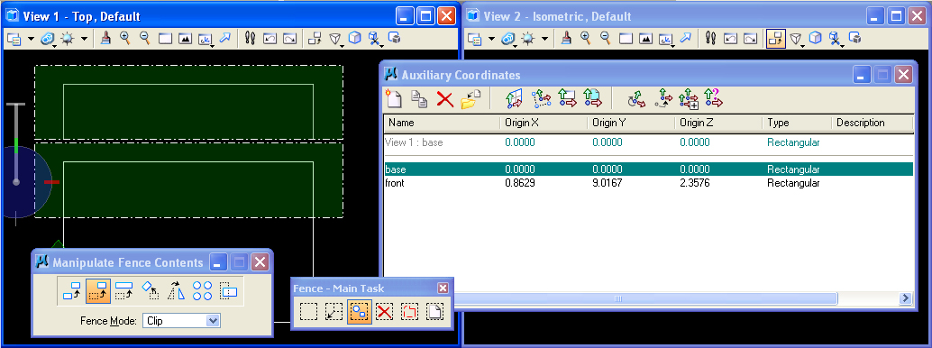
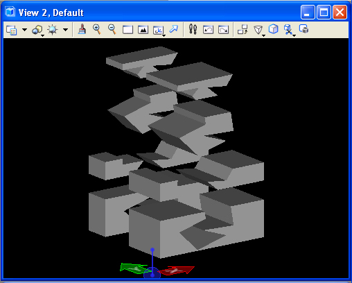
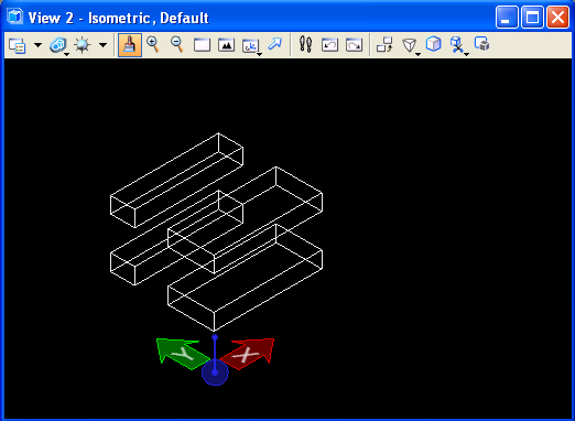
The
result
of the preceding two operations is to splice the slab into four slabs.
Note that the fence tool in the top view operates on upper
visible slab as well as the occluded lower slab in that view.
That is, the fence projects the operation entirely through every object
in its pathway in that view.
2.
STRETCH
OPERATION
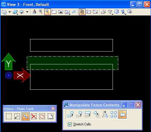
Re-select
the front view, then select the "front" ACS in the Auxiliary
Coordinates dialog box, and place the fence over the slabs in
the
lower portion of the view window. Next use the "Manipulate
Fence Contents" and "Stretch" tool option (shown
below) to
change the
height of the cubes on the ground plane..
Once
again,
the fence projects the operation entirely through every object
in its pathway in that view and they are stretched to have a larger
"Y'" dimension. Note that a truncated cone (not shown) in similar situation would also have stretched in a tapering
way preserving its tapering geometry. Similarly, other objects will also stetch appropriate to their
geometry.
3.
NON-RECTANGULAR FENCE
Select the "Front" view and then the "front: ACS from the Auxiliary Coordinates Dialog box. Next, select
the" Fence"
tool,
change the fence type to "Shape", and
draw an
arbitrary polygon over the front view.
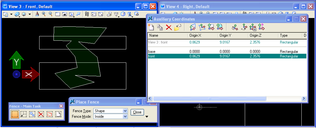
Zoom out of the
"Front" view
and use the "Manipulate Fence Contents/Move" option to clip the
arbitrary shape to a location above the slabs. Note that the operation
cuts the arbitrary shape out of the cubes and moves it above them.
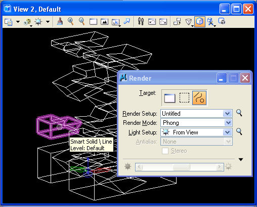
3. RENDERING WITH THE
FENCE TOOL
In View 2, draw a "block"
Fence
over a portion of the view window. In the Visualization task, adjust
the solar lighting using the W1 tool, select the "Render"
(Q1) tool, and choose the "Fence" option. The result is that
a
smaller sample portion of the view window is rendered. This can be a
very efficient way to sample the rendering quality without having to
expend much greater time in testing the entire view window. Note that
rendering 1/4th of the view window in Ray Trace will be significantly
faster than doing the whole view.
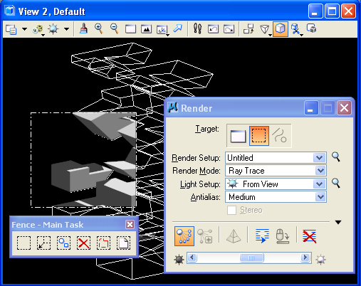
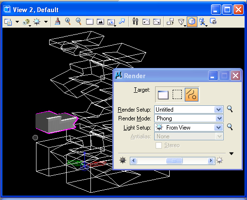
Note that the Render
dialog box
also allows you to render individual objects in several render modes,
such as Phong or Smooth shading. This is achieved by selecting the
third icon in the "Render" dialog box as depicted below. However, this
doens't work in Ray Trace mode (since the rendering algorithm is based
on backward tracing of rays for every pixel in the rendered area).
PART
II: EDIT BY
SURFACE PROJECTION
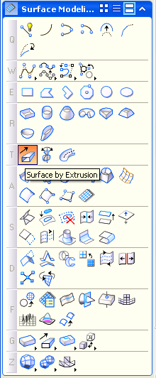
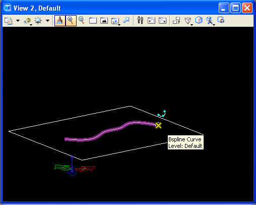
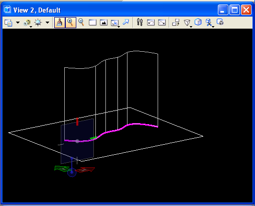
Erase
the current elements in the
model, and place a rectangular block and a bspline curve in the ground
plane. Next, within the Solids task, use the projection tool (T1)to project the bspline
curve into the vertical direction.
Place a slab in the model so that it is fully encompassed by the new
surface.
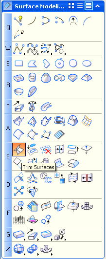
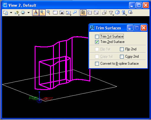
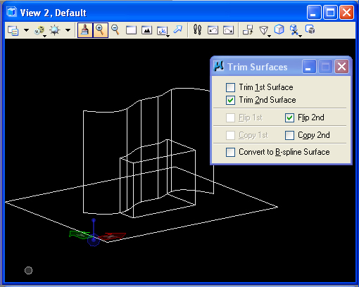
In the Surfaces task, sleect the "Trim Surfaces" tool (S1) and select
the
"Trim 2nd" option, then pick the surface first and the slab second.
Enter an additional data point in the view window to initiate the trim
and a fourth data point to confirm it. Note that a portion of
the
slab is trimmed away.
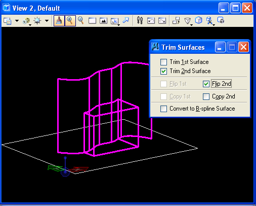
The reverse part of
the slab is trimmed away if the "Flip 2nd' option is turned on.
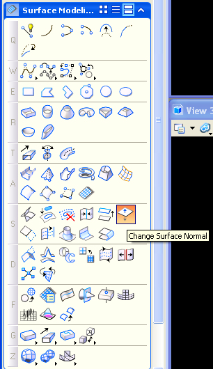
The
surface trims the slab according
to the direction of its surface normal vector (the positive side of the
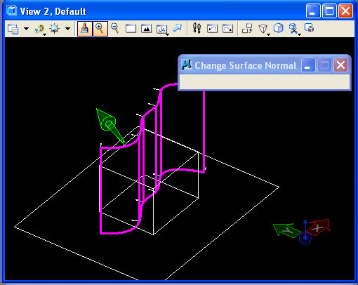
surface). This vector can be reversed through the use of the "Change
Surface Normal" tool(S6) in the "Surfaces" task(image at left below). Selecting the green
surface normal arrow will reverse its direction. Completing this step
and re-doing the trim surface operation will reverse the portion of the
slab that is trimmed away.
PART
III: GC FUNCTION EXAMPLES (EXTRACURRICULAR)
The
two examples presented here go slightly beyond the scope of our basic
introduction to generative components and incorporate "function" update
methods that contain "while" loops.
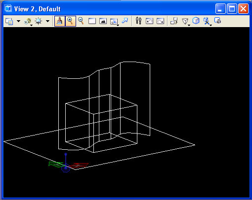
1. Spiral
The GC
example
spiral2.gct draws and archimedes
spriral that can be transformed into an accelerating spiral. A number
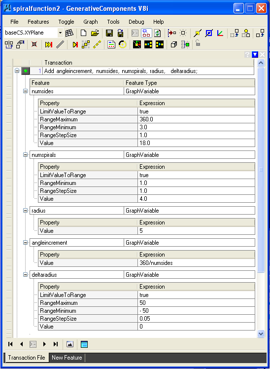
of graph variables are
defined in
the first
step of this GC file according to the methods examined in earlier
workshops. The variables determine the resolution, scope and size of
the spiral:
numsides = number of sides in each 360 degree spiral
numspirals = total number of 360 degree spirals
radius = radius of initial spiral
angleincrement = incremental angular distance between points in a given
spiral ( = 360 / numsides)
deltaradius = accelerating rate for the radius from spiral to spiral
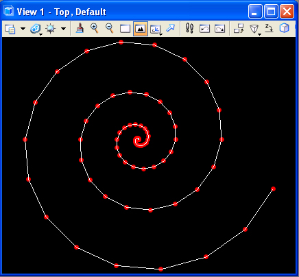
Note that if deltaradius = 0, then the spiral is an archimedes spiral.
If delatradius > 0, then the spiral accelerates.
In the second
step, the GC file incorporates a polygon line " Function" update
method, essentially a short algorithm that handles the generation of
the spiral.
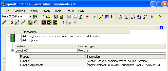
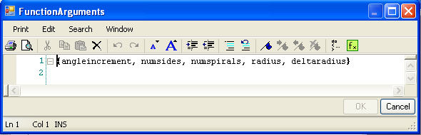
When placing the
mouse in the textbox containing the function arguements
"{angleincrement, numsides, numspirals, radius, deltaradius}", the
function arguments can be more closely examine by selecting the text
editing icon (a small rectangle next to the "fx" symbol) that appears on the right hand side of the "FunctionArguements" textbox below.
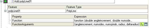
Note that the arguments are set off by a left and right curly bracket.
These are the same variables that were defined in the first step of the GC
file.
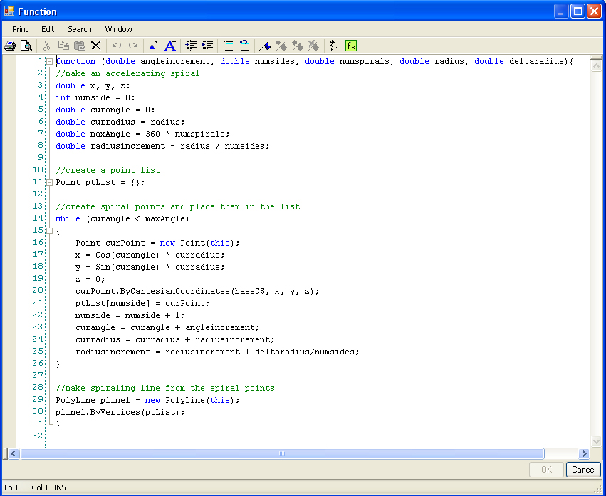
SImilarly, when placing the mouse in the Function textbox adjacent to the words "Function (double
angleincrement, double numside ... }, the function update
method can be examined more closely. The details of this function are
somewhat beyond the intentions of this quick summary, and so a brief
overview is given here only.
The arguments to the function are all given a type "double" declaration
in that they are decimal numbers. Additional integer "int"
and "double" variables are defined internal to the function. The update
method
incorporates a "while" loop that continues to repeat when "curangle" of
the radial point tracing out the spiral is less than then "maxAngle",
the maximum angle of the final point in the spiral. Note
that "maxAngle = 360 * numspirals". Inside the "while" loop,
as the point travels around the center of the spiral, the
current angle and radius is continually updated. Each new point in the
spiral is stored in a Point array named "ptLlist" . Thus, the first
point is stored in "ptList[0]", the second point is stored in
"ptList[1]" and so on. When the loop is concluded, a polyline
is created from the listing of points.
The use of
iterative loops can efficiently express a
condition in which an action is repeated continuously as is used to
draw
the spiral. Note, if the variable
"deltaradius" is equal to 0, then the result of the above function is an
Archimedes spiral.
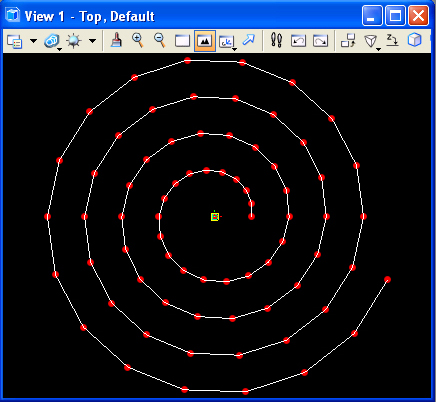
If the variable ""deltaradius" is greater than
0, then the spiral becomes accelerating one.
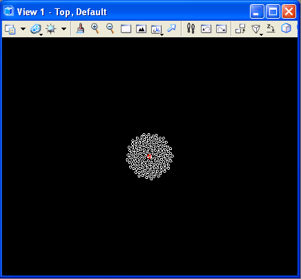
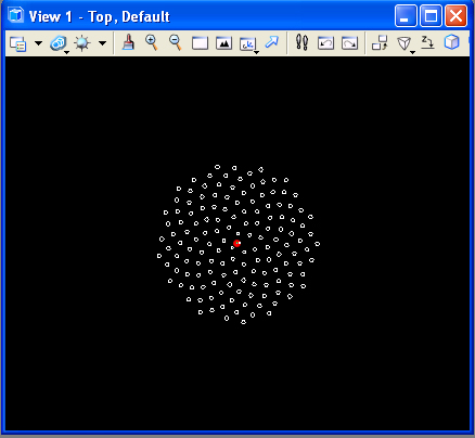
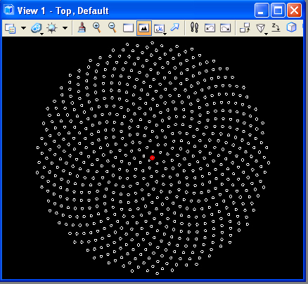
2. Daisy head
Similarly, the example file daisyseedfromFermat.gct
incorporates a de-accelerating spiral according to a theorem by the
mathematician Fermat. That is, the basis for the geometry is a Fermat
curve. The code for this example after an algorithm initially published by Dixon. Placed
along the loop are polygons that capture the pattern of seeds in a
daisy head. The variables for the transaction file can control the
tightness of the seeds together and the number of spirals as
illustrated in the following three images.
 |
 |
 |
| tightness is
high, number of spirals is low |
tightness is
low, number of spirals is low |
tightness is
low, number of spirals is high |