COMPUTER AIDED
ARCHITECTURAL DESIGN
Workshop 7 Notes,
Week of October 18, 2010
Editing by Projection, Fence Tools, Cutting Solids with Surfaces
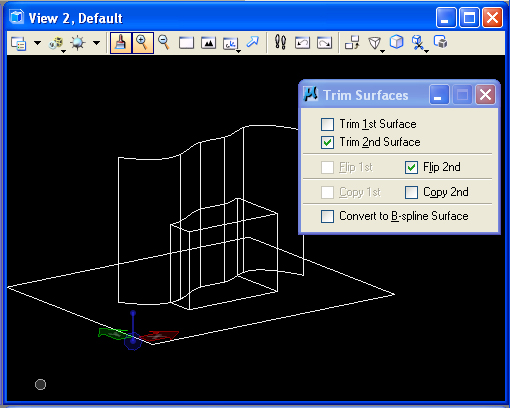
Most of these tools operate through projection of one geometry onto another. A few tools, such as the trim surface tools, allow you to cut solids with doubly curved or planar surfaces. Note that surfaces have a positive and negative side which can impact the cutting action that they peforrm. The positive and negative directions can be reversed. This workshop will also re-introduce the creation of construction planes through the Auxilliary Coordinates Dialog Box
PART
I: FENCE TOOLS
|
|
|
|
|
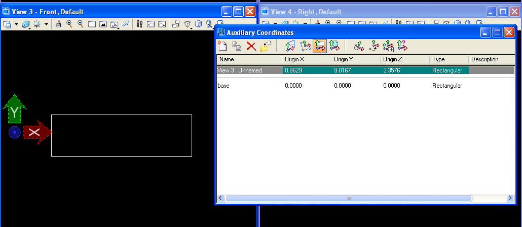
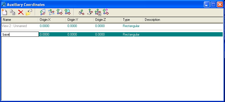
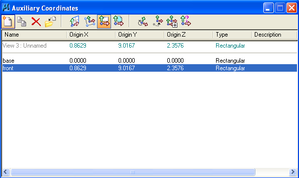
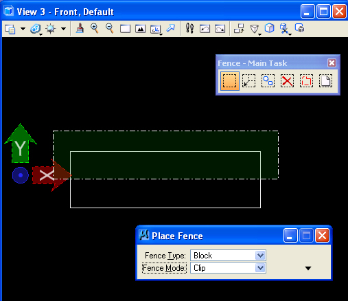
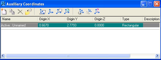
Save the new ACS as "front" within the Auxiliary Coordinates
dialog box.
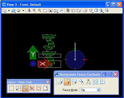
Open the fence tools subpalette from the main task menu (#2 key).
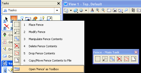
Draw
a
"Fence" in the front view window with "Fence Mode" set to
"Clip". This mode
isolates what's inside the fence from the outside.
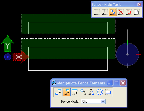
Select the "Manipulate Fence
Contents Icon" (second icon in the Fence palette) andnthe "Move"
option, and enter two data points in the front view with to
clip off and move upward
the geometry that is encompassed within the fence.
Similarly, select the top view
window. Select the "base" ACS form
the
Auxiliary Coordinates Dialog box, and repeat the same move
operation on the upper "Y" axis portion of the cubes from the top view.
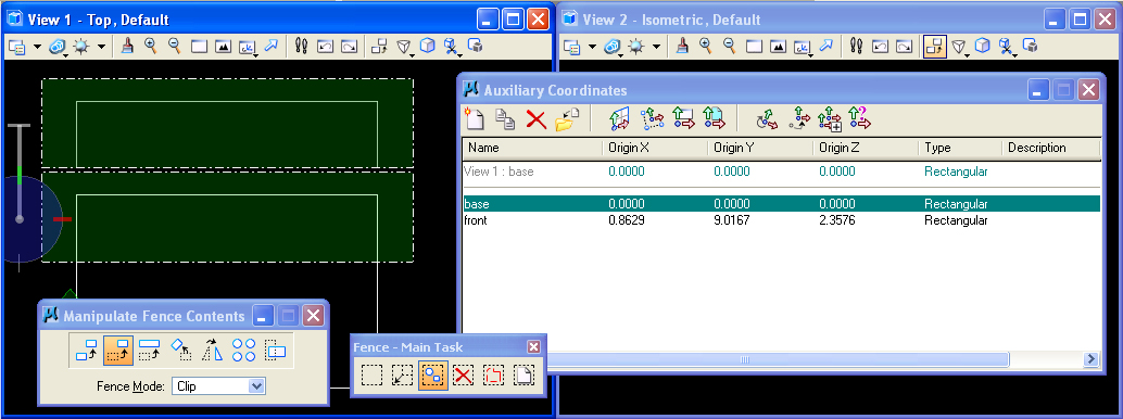
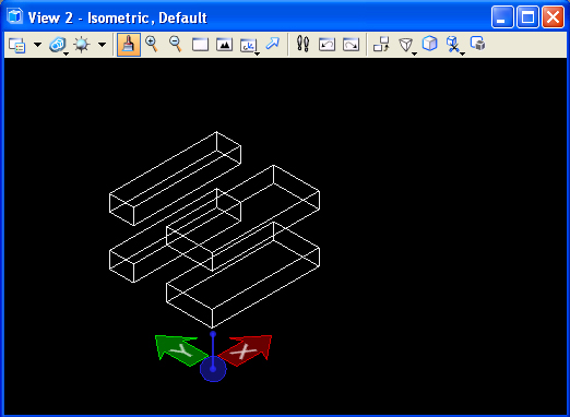
The result of the preceding two operations is to splice the slab into four slabs. Note that the fence tool in the top view operates on upper visible slab as well as the occluded lower slab in that view. That is, the fence projects the operation entirely through every object in its pathway in that view.
2.
STRETCH
OPERATION
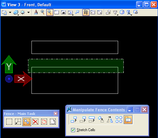
Re-select
the front view, then select the "front" ACS in the Auxiliary
Coordinates dialog box, and place the fence over the slabs in
the
lower portion of the view window. Next use the "Manipulate
Fence Contents" and "Stretch" tool option (shown
below) to
change the
height of the cubes on the ground plane..
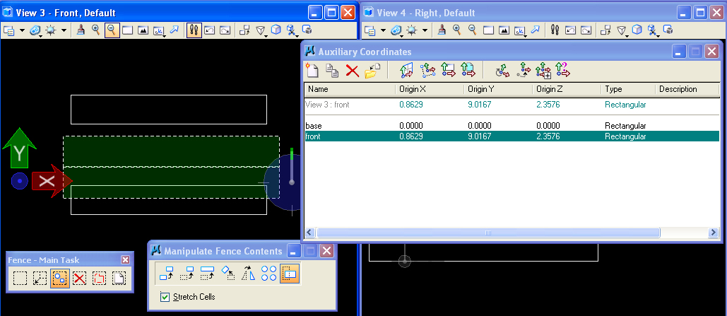
Once again, the fence projects the operation entirely through every object in its pathway in that view and they are stretched to have a larger "Y'" dimension. Note that a truncated cone (not shown) in similar situation would also have stretched in a tapering way preserving its tapering geometry. Similarly, other objects will also stetch appropriate to their geometry.
3. NON-RECTANGULAR FENCE
Select the "Front" view and then the "front: ACS from the Auxiliary Coordinates Dialog box. Next, select the" Fence" tool, change the fence type to "Shape", and draw an arbitrary polygon over the front view.
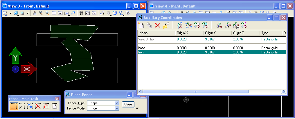
Zoom out of the "Front" view and use the "Manipulate Fence Contents/Move" option to clip the arbitrary shape to a location above the slabs. Note that the operation cuts the arbitrary shape out of the cubes and moves it above them.
 |
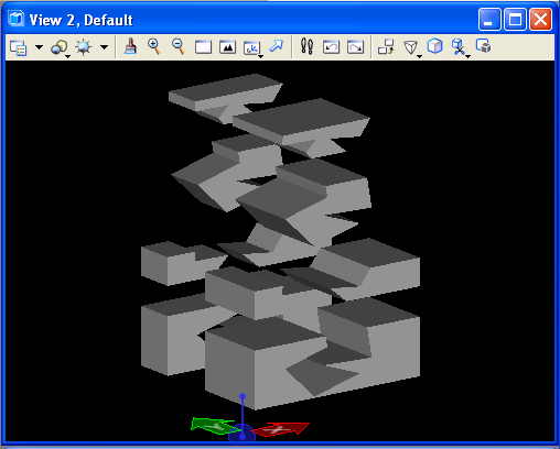 |
3. RENDERING WITH THE FENCE TOOL
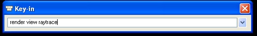
The technique involves using a "key-in command". Go to the "Utilities/Key-in" menu and enter the command "render view raytrace" followed by the "return" key.
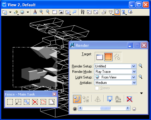
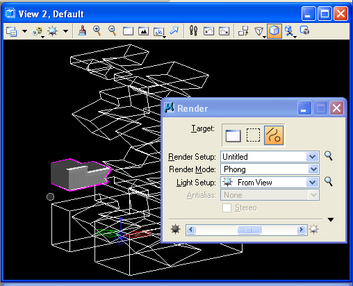
In View 2, draw a "block" Fence over a portion of the view window. In the Visualization, adjust the solar lighting using the W1 tool, select the "Render" (Q1) tool, and choose the "Fence" option. The result is that a smaller sample portion of the view window is rendered. This can be a very efficient way to sample the rendering quality without having to expend much greater time in testing the entire view window. Note that rendering 1/4th of the view window in Ray Trace will be significantly faster than doing the whole view.
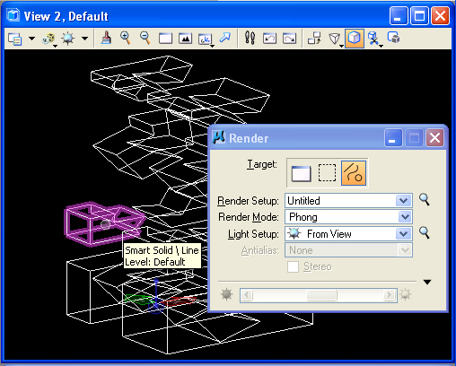
Note that the Render dialog box also allows you to render individual objects in several render modes, such as Phong or Smooth shading. This is achieved by pre-selecting the object you wish to render. Use the key-in command "Render View Phong" and then selecting the third icon in the "Render" dialog box as depicted below. Note that, this doens't work in Ray Trace mode (since the rendering algorithm is based on backward tracing of rays for every pixel in the rendered area.
 |
 |
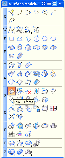
PART II: EDIT BY SURFACE PROJECTION
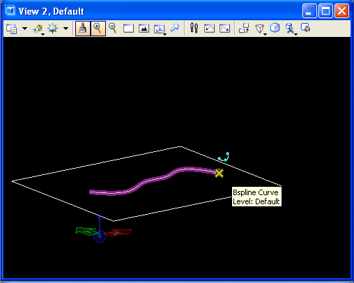
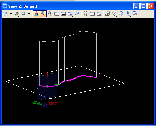
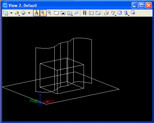
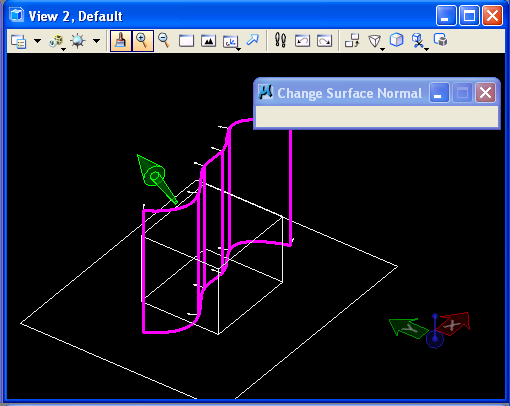
Erase the current elements in the model, and place a rectangular block and a bspline curve in the ground plane. Next, within the Solids task, use the projection tool (T1)to project the bspline curve into the vertical direction.
 |
 |
 |
 |
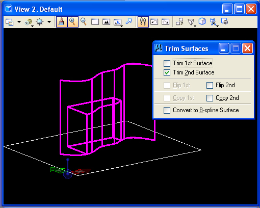 |
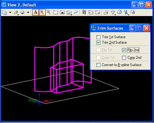
The reverse part of the slab is trimmed away if the "Flip 2nd' option is turned on.
 |
 |
 |
 |
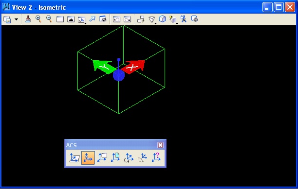
4. . ACS and ACCUDRAW (POSSIBLY SKIP UNTIL NEXT WEEK)
ACS and ACCUDRAW are two inter-related but two distinct ways of establishing construction planes. The ACS, Auxilliary Coordinate System, is set into place on a more continuous basis and can be moved into any location and orientation. ACCUDRAW, a consturction plane compass, is set into place on a more transitory basis, and can be very quickly rotated and setup in relationship to the the active ACS. The combination of both systems affords quick and contextually sensitive options to build construction planes as needed.
ACS = Auxilliary
Coordinate System. The ACS is the active construction plane, a two
dimensional plane on which you create data points.
ACCUDRAW = The Accudraw Compass. The ACCUDRAW compass is a construction
plane that is defined in relationship to the ACS. It is accssible
through a set of QUICK KEYS (e.g, "F" - front, etc.). By default, it is
co-planar with the ACS.
5. ACCUDRAW AND AUXILLIARY COORDINATE SYSTEM (ACS) REVISITED
1. 2d plane rotate 90 degrees on any axis (draw circles, arcs, etc.) (QUICK KEYS: "RX", or "RY", or "RZ")
Enter the first data point on the current Accudraw construction plan, enter the letter "O" for offset, and then use one of the following quick key combinations to rotate Accudraw around the x, y, or z axis:
Accudraw via "RX" key transforms to rotation of 90 degrees around x-axis.
Accudraw via "RY" key transforms to rotation of 90 degrees around y-axis.
Accudraw via "RZ" key transforms to rotation of 90 degrees around z-axis.
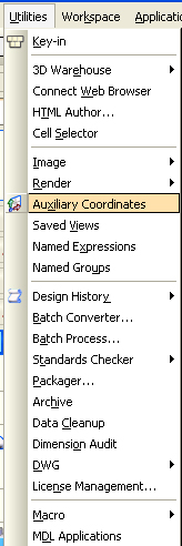
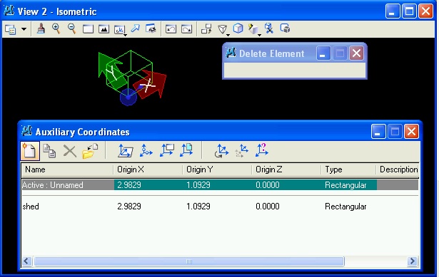
2. Menu item utilities/auxiliary coordinates for ACS options:
2.1a The current ACS can be saved under a named identity with the "Create new ACS icon"
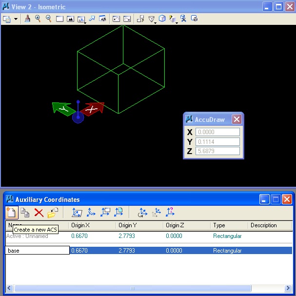
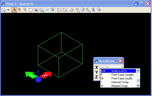
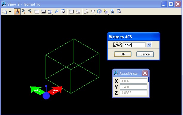
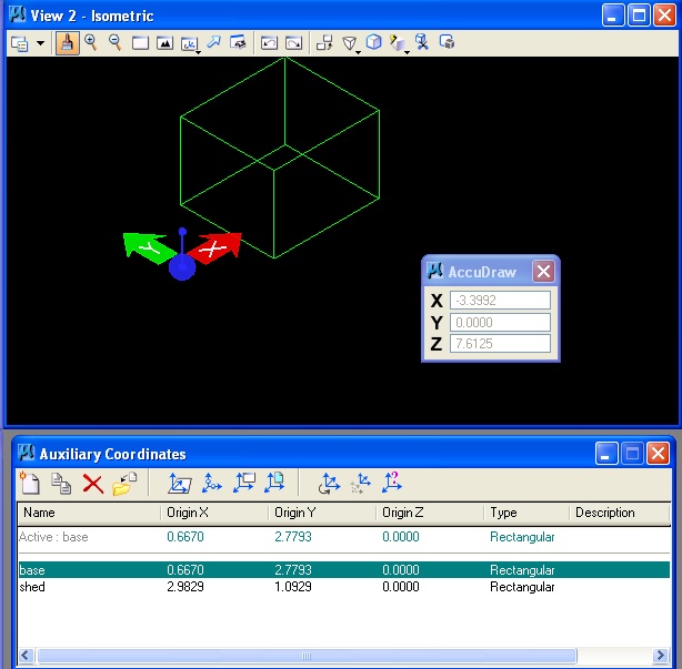
2.1b Alternatively, save “base”
(default ACS) via Accudraw by selecting Accudraw dialog box and using the quick key combination "WA"
2.2 Redefine ACS (three point method). Note that the red and green arrows are rotated into the new position.
2.3 Similar to example 2.1, we can use the save the current ACS as “shed":
2.4 Double-clicking on “base”
restores the ACS "base":
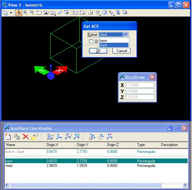
2.5 Alternatively, using Accudraw, the quick key combination "GA" restores ("gets ACS") the ACS "shed":
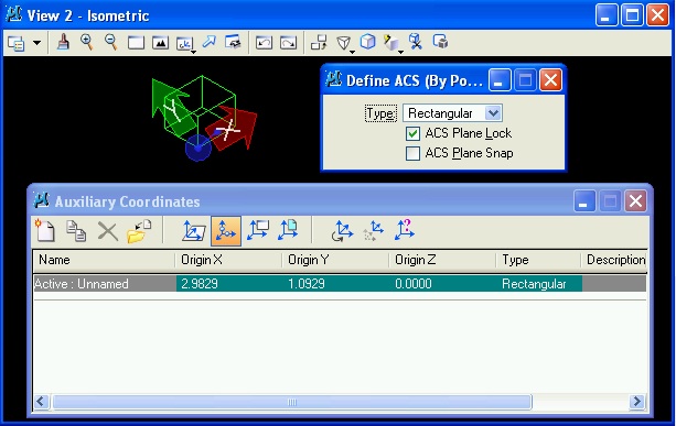
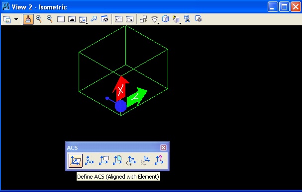
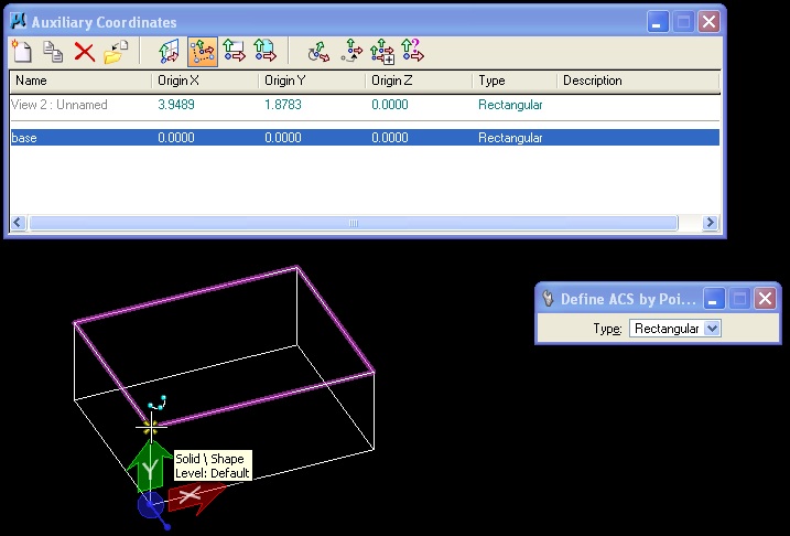
3. ACS via TOOLS Menu
Menu item tools/auxiliary coordinates obtains a separate dialog box thatalso allows the following ACS operations:
icon 1: define acs with element (select front rectangle of cube, fix acs to it.
icon 2: define acs with 3 points (on face of cube)
The remaining icons reset the ACS as follows:
icon 3: align acs with view
icon 4: align with attached reference file (skip)
icon 5: rotate it by value
icon 6: move it (if time)
icon 7: select ACS (similar toquick key "GA”)
4. CUTTING SOLID WITH DOUBLY CURVED SURFACE
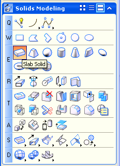
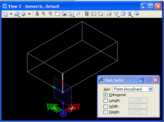
4.1 In the Solids Modeling task, create a Slab Solid with the "E1" tool.
4.2 Using Auxiliary Coordinates Menu, determine an ACS with three points on front face of the cube.
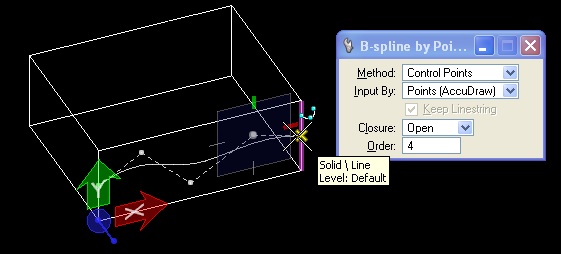
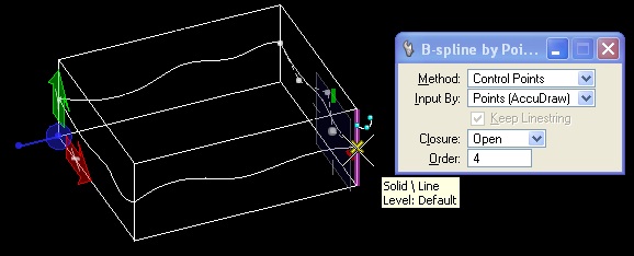
4.3 From the Solids Modeling task, using the "Q3" tool,
add a B-spline by Points from the mid-point of the left-hand edge to the mid-point of the right-hand edge of the front face of the slab..
4.4 Simillary, using the same ACS, add a B-spline by Points to the rear face of the Solid Slab.
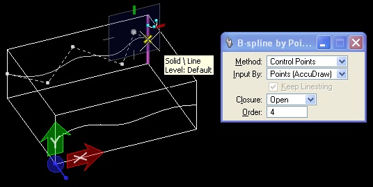
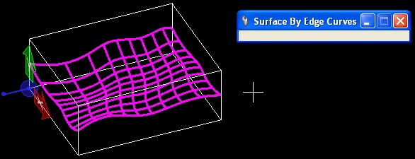
4.5 Change the ACS to the left-side of the Solid Slab, and add two additional B-splines linking up to those on the front an rear faces.
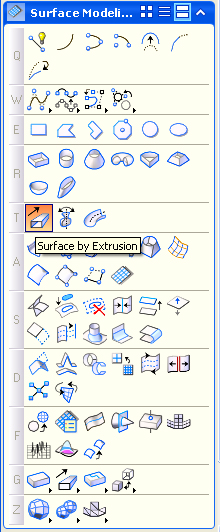
4.6. Working from the Surface Modeling task, pre-select the four B-splines, and then choose the "A7" Surface by Edge Curves tool to create a doubly curved surface.
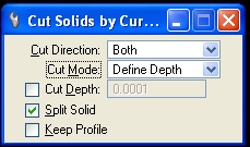
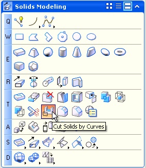
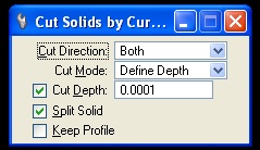
4.7 In the Solids Modeling task, use the "T11" Cut Solids by Curves" tool, set the parameters to "Cut Direction" = "Both", "Cut Mode" = "Define Depth", select on "Cut Depth" and set is value to a nominal 0.0001, and select on "Split Solid".
4.8 Select the Solid and then select the Surface, and enter a data point to split the solid and another to confirm it.
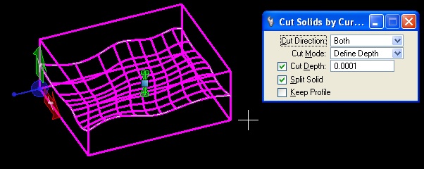
4.9 The result is that the solid slab is devided into an upper and lower part.
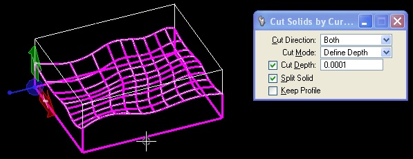
4.10 Alternatively, choose the "Cut Mode" = "Define Depth" option, but do not select the check-box for the "Cut Depth" option, enter the data points needed to generate split and confirm it, and the solid will split without any depth between upper and lower parts.