1. Introduction
Grasshopper
is a
graphical programming environment. It provides an associative
geometrical modeling tool with constraints.
It is associative
in the sense that the state of one element is
linked to the state of other elements. A constraint
is a designed restriction on how elements may be associated. For a
simple example, a door may be associative
with an opening in a wall. The resizing of a door may be automatically
linked to the resizing of the opening in a wall. A door may also have constraints.
For example, the door may restricted to be in some alignment with a
window in an opposite wall.
Grasshopper can also be partially parametric.
That is, returning to and revising
a few decisions made early in a construction sequence of a Grasshopper
document automatically
re-propagates the geometry established in later steps. One industry
expert,
Robert Pierce, described a parametric process as one having an
"editable history". (A more complete parametric system would
likely extend the ability to automatically update changes to geometry
that has been transferred from Grasshopper into Rhino. This point
is slighltly beyond the scope of this first workshop and will be taken
up later.)
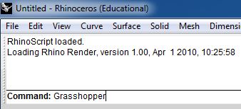
Grasshopper is available as a third party plugin that can be downloaded from the Rhino Web site. Follow the instructions on the Rhino3d.com web site for downloading and installing the software. Note that the examples used here are based on the version of August 2013 Earlier versions of Grasshopper may not be compatible. To begin, type in "Grasshopper" at the command prompt in Rhino.
This first hands-on introduction of Grasshopper will demonstrate the concepts needed to construct some basic geometrical elements. Next, in a later set of workshop notes, we will look at writing a short algorithm with the Python plugin to Grasshopper.
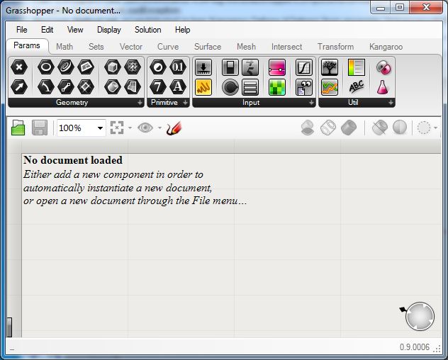
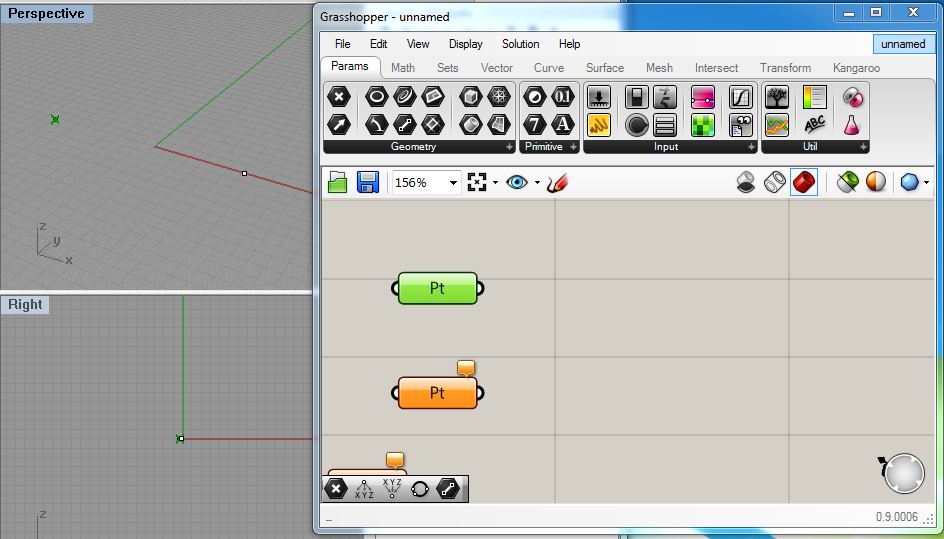
This opens up the Grasshopper dialog window. Note that there are a number of tabs in the dialog window, including the "Params" tab active below. These tabs contain different sets of components. The "Params" tab provides components for inputting data into Grasshopper.
1.1 Building A Simple Line
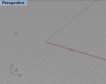
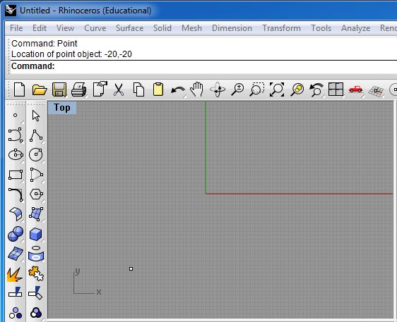
To initiate a simple line, draw two points in the XY plane in Rhino.
Now within Grasshopper, left click on the "Point" param (the "X" component in the upper left-hand corner of the Params options) and drag two copies into the work area.
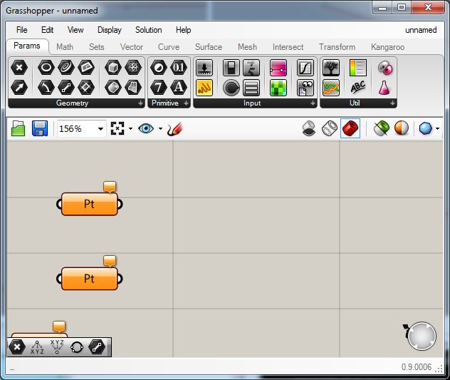
Next, within the Grasshopper Window right click on the first point component labelled 'Pt", go to the "Set One Point" option with the left mouse button, and then draw a small window around the first of the two points in the Rhino Perspective window. Repeat the same process for the second point labelled "Pt". When select either "Pt" component in Grasshopper the corresponding point inside the Rhino window in turn is highlighted with a green "X" mark.
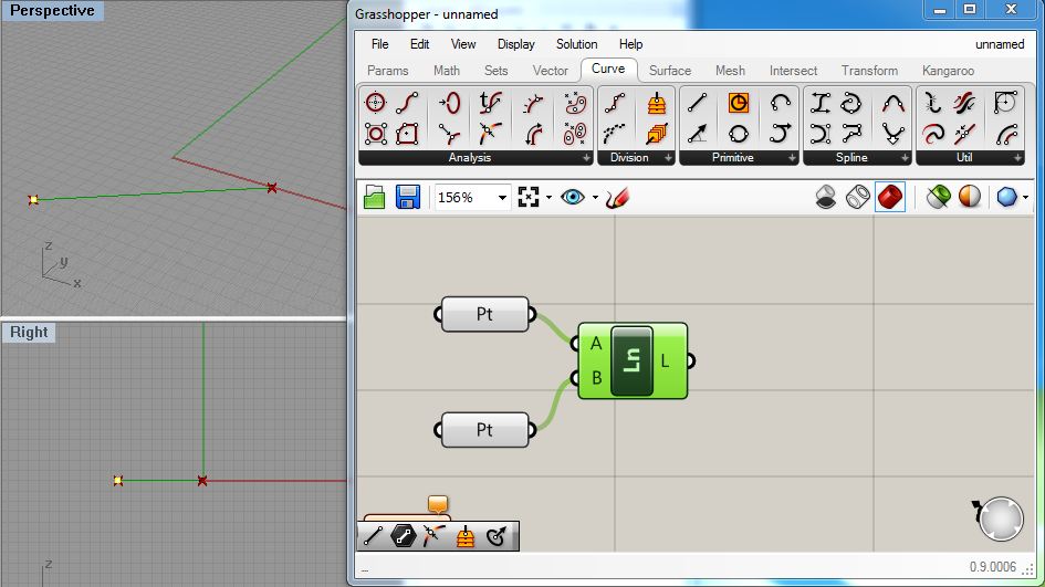
Next, with the left-mouse button connect the output port of the of the first point to the "A" input port of the line. Similarly connect the output port of the second point with the "B" input port of the line.
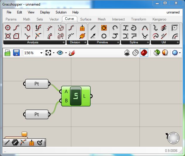
Note that the line now appears in the Rhino view window, and that if you move any of the original two input points directly in Rhino, the line is automatically redefined accordingly.
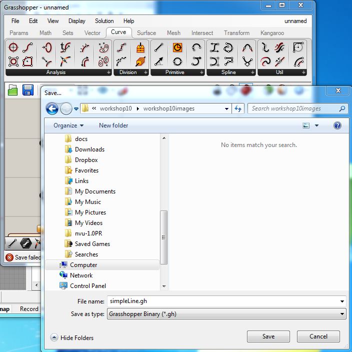
To save the Grasshopper file, go to "File/Save" in the upper-left hand corner of the Grasshopper dialog box and save the file to some <filename>.gh (e.g., "simpleLine.gh").
1.2 Adding a parametric point to the line.
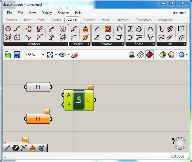
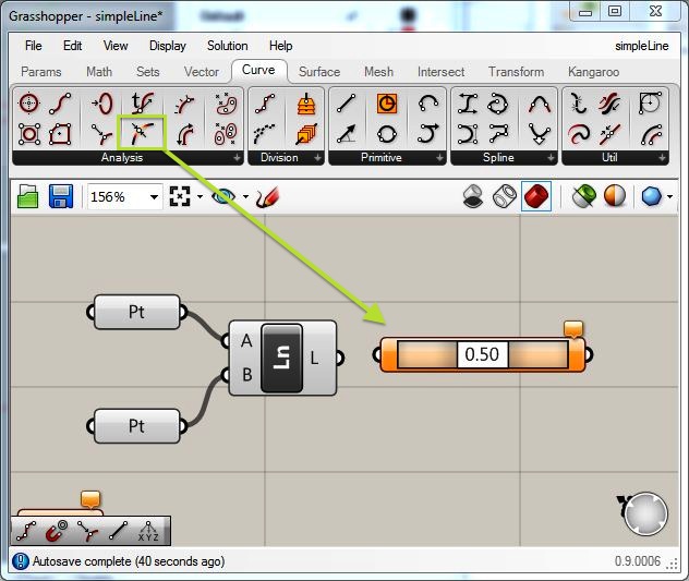
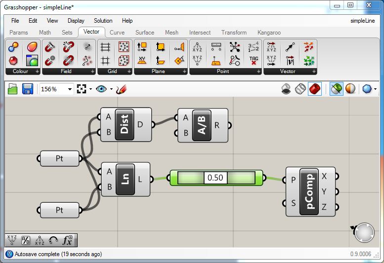
Building upon the line, go to the components in the "Analysis" part of the "Curve" tab, and with the left-mouse button select the "point on curve" icon and drag into into the Grasshopper work window just to the right of the "Ln" component.
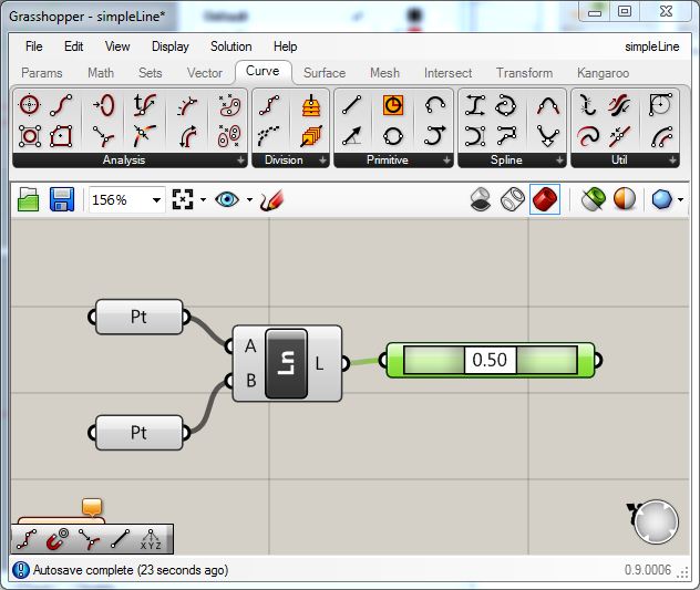
Next, with the left-mouse button connect the output port of the line "Ln" component to the input port of the "point on curve" component. A point will now appear on the line in the Rhino view windows.
The value of the slider within the "point on curve" component ranges from 0.0 to 1.0 and represents the percentage distance of the point along the line from "A" to "B", the original two points that define the line. Thus a value of 0.25 is one fourth of the distance from A to B.
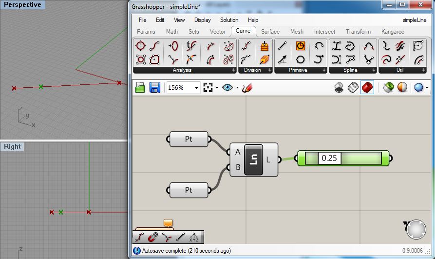
Thus, the construction of the figure is rigged such that any changes to the original two points will change the length and direction of the line, and in turn, adjusting the parameter (i.e., 0.25) of the point on the line will shift its position along the line. Similarly, other components and numerical values can be added to and associated with the elements of this construction to produce a more complex geometrical form.
1.3 Defining a vertical arc based upon the original two end points and the point on the line.
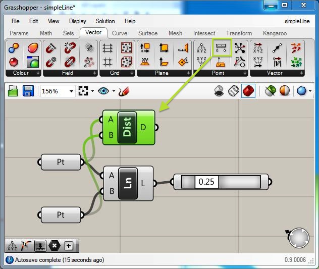
In order to build an arc above the line, we first measure the distance between the two end points. Go to the "Vector" tab and in the "Point" area select the "Distance" component (looks like a ruler with two points below it) and place it in the Grasshopper work window just above the "Ln" component. Connect the output ports of the original two points to two inputs of the "Distance" component.
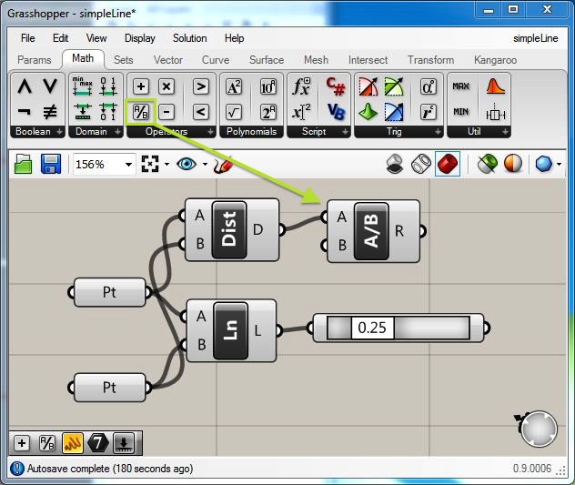
Now, go to "Math" tab and in the "Operators" area select the "A/B" component and place it in the Grasshopper work window just to the right of the "Distance" component. Connect the output port of the "Distance" component to input port "A" of the "A/B" component in order to provide the numerator for the division. Right-click on the "B" port of the "A/B' component, go to the "set data item" option, and add the value "2.0" in order to provide a denominator for the division. We will use the result "R" of the division as the radius of the arc.
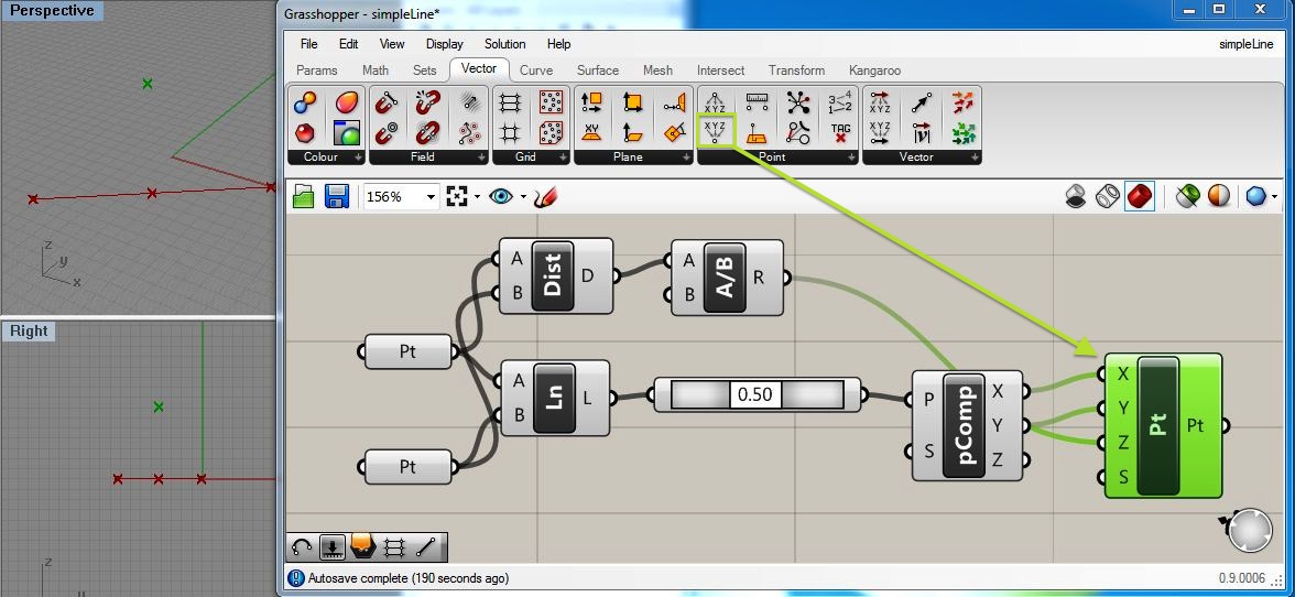
The original two points of this construction sequence will determine the end points of the arc. Given a radius, and a point midway between the first two points, we can determine a third point which lies on the arc above the ground plane. Go to the "Vector" tab and in the "Point" area select the "Decompose" point component and place it in the Grasshopper work window just to the right of the "point on curve"component.
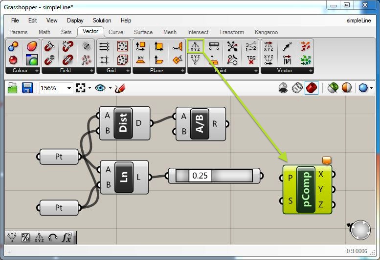
Connect the output port of the "point on curve" component to input port "P" of the "Decompose" component.
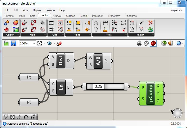
Now, we are going to set the parametric value of the "point on curve" to 0.5 so that it lies at the center of the line.
Next, go to the "Vector" tab and in the "Point" area select the "Point" component and place it in the Grasshopper work window just to the right of the "Decompose" component. Connect the output port "X" of the "Decompose" component to the input port "X" of the new "Point" component. Similarly, connect the output port "Y" of the "Decompose" component to the input port "Y" of the new "Point" component. Howeve, to get z-value of the interior point on the arc, connect the output port "R" on the division "A/B" component to the input port "Z" of the new "Point" component. This creates a new arc point above the point on the line.
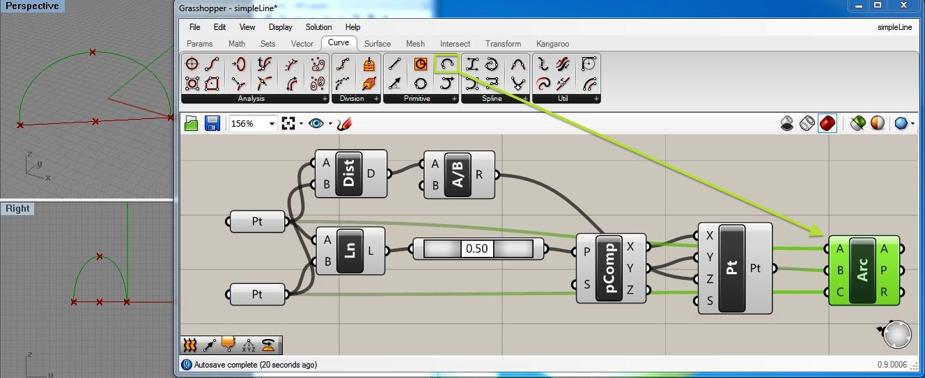
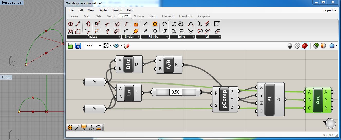
Finally, go to the "Curve" tab and in the "Primitive" area select the "Arc3Pt" component and place it in the Grasshopper work window just to the right of the recently added "Point" component. Connect the the output port of the original first point to the input port "A" of the "Arc3Pt" component. Connect the the output port of the original first point to the input port "C" of the "Arc3Pt" component. Now, to fully determine the arc, connect the the output port "Pt" of the new arc point to the input port "B" of the "Arc3Pt" component, and it will generate the arc.
Note that we have retained the entire chain of events in the component diagram that is inside the Grasshopper work window. If you go to Rhino and move one of the original end points of the arc, then in turn 1. the line between the two end points is changed, 2. the point interior to the line is thus changed, 3. the interior point on the arc is changed, and 4. the arc itself is changed. That is, we have made entire construction sequence open to direct modification at any step along the way.
2. ALGEBRAIC EXPRESSIONS
GIven a grid of points, a direct and concise algebraic expression can be used to define a surface topology. Whereas in the prior example, each point on the arc required an explicit component to hold the data or to perform a mathematic operation, here we can use sets of data to compress the number of steps need to build a geometrical construction.
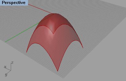
EXAMPLE 1. Hyperbolic parabolic surface from a simple two-dimensional array.
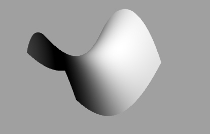
We begin by establishing a point grid on the ground plane. We then use the equation of a hyerbolic parabolic surface to establish a point at a vector distance from each point on the ground plane.
Step 1: Create a point at the location -20, -20 in the XY Plane
Step 2: Use rectangular grid as described in the table below.
To create a rectangular grid within the x, y plane and beginning the the point -20, -20, we need the following information
| Point -20,20 | Defines the origin for the grid |
| Sx -size grid cell on x-axis | 1 |
| Sy - size grid cell on y-axis | 1 |
| Ex - number of grid cells on x-axis | 40 |
| Ey - number of grid cells on y-axis | 40 |
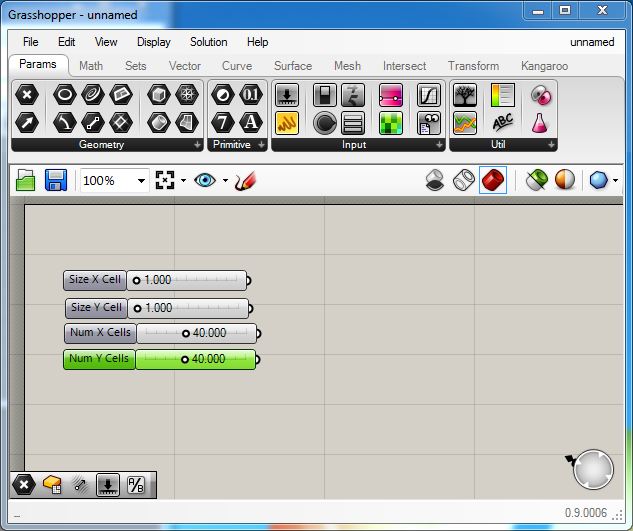
Therefore, working in Grasshopper go to the "Params" tab and in the "Input" area select the "Number Slider" and place four copies in the work window.
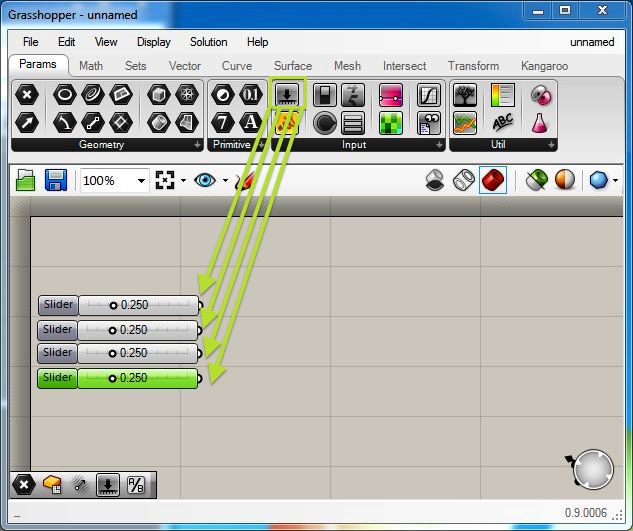
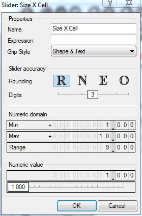
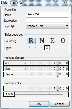
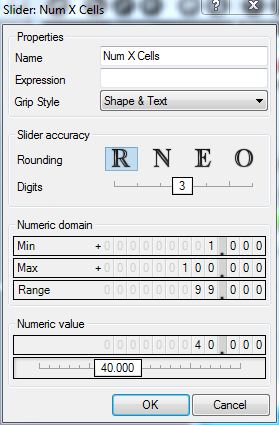
Double-click on the left-side of each slider and directly on the text "slider" to edit each one. Rename each of the four sliders and revise the their range of values according to the table below.
Slider Name
Min
Max
Range
Numeric
Value
Size
X Cell
1
10
9
1
Size
Y Cell
1
10
9
1
Num
X Cells
1
100
99
40
Num
Y Cells
1
100
99
40
 |
 |
 |
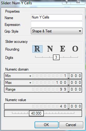 |
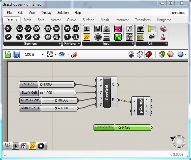
The revised appearance of the slider in the Grasshopper work window now appears as follows:
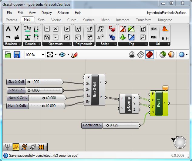
Now, go to the "Vector" tab and in the "Grid" area select the "Rectangular" grid component and place it in the Grasshopper work window to the right of the numerical sliders.
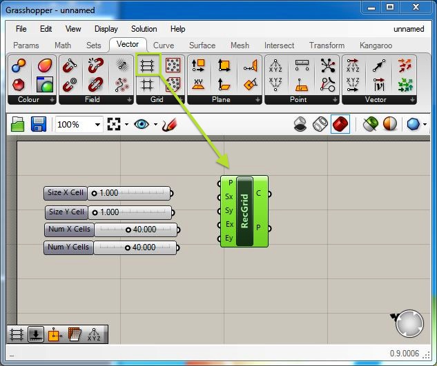
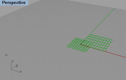
Note that the new grid is displayed in Rhino initially at the origin of the XY ground plane.
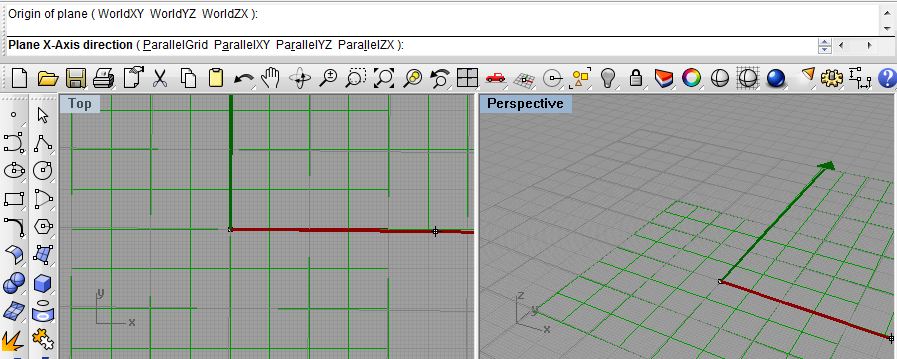
Next, right-click on the input parameter P and a) select the "set one plane" option and set it to the point at -20,-20 created earlier in Rhino, and b) in the Rhino command prompt area choose the "ParallelXY" modifier.
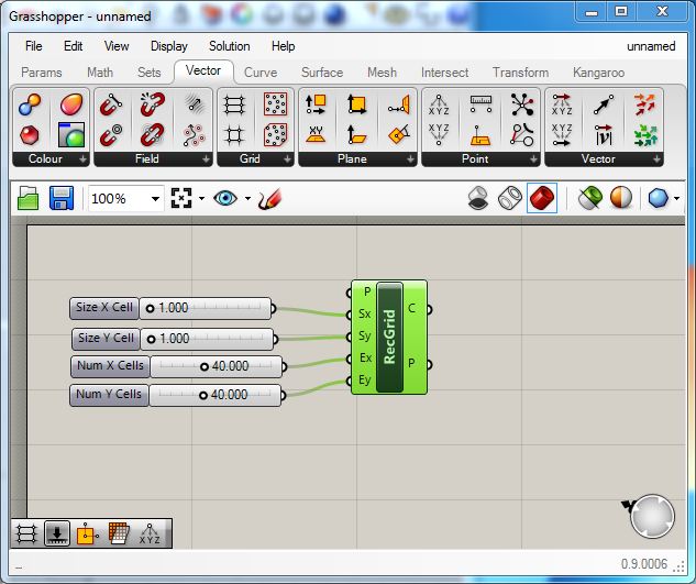
In addition, connect the output ports of the numerical sliders to the input ports Sx, Sy, Ex, Ey of the "Rectangular" grid component as follows:
Step 3: Add point at a vector direction (Zdirection) and distance (hyperbolic parabolic equation) to each point on the Grid
More
specifically, for each point P on the in the rectangular grid with
Cartesian coordinates x, y, z, the next step is to create a point
determined by a scalar coeficient "s" and the hyperbolic parabolic
expression (x2
- y2).
| P | point in the x-y rectangular grid |
| x | x coordinate value of P |
| y | y coordinate value of P |
| s | scalar coeficient ranges in value from 0.0 to 2.0 |
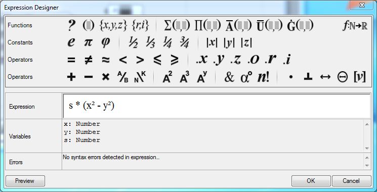
| Height of point above P | s * (x2 - y2) |
First, we
need to strip out the x, y values of each point on the grid. Go
to the "Vector"
tab and in
the
"Point" area select the "Decompose" point component
and place
it in the
Grasshopper work window to the right of the "RecGrid"
component.
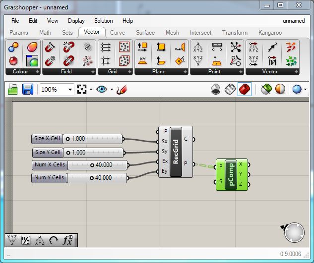
Next, connect the output port "P" of the "RecGrid" component to the input port "P" of recently added "Decompose" point component.
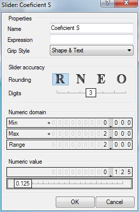
Next, returning to the "Params" tab, add a "Number Slider" for the coeficient "S" and set its values to a minimum of 0 and maximum of 2 for an overall range of 2, and also set its current value to0 .125.
 |
 |
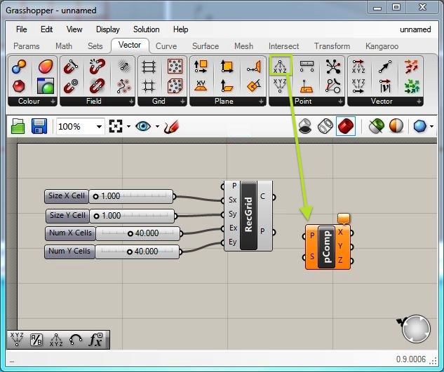
Next, go to the "Math" tab and in the "Script" area select the "Fx" function component and place it in the Grasshopper work window to the right of the "Decompose" point component.
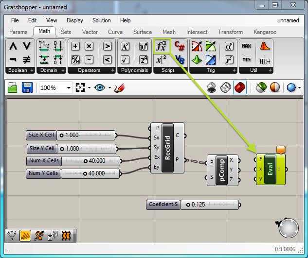
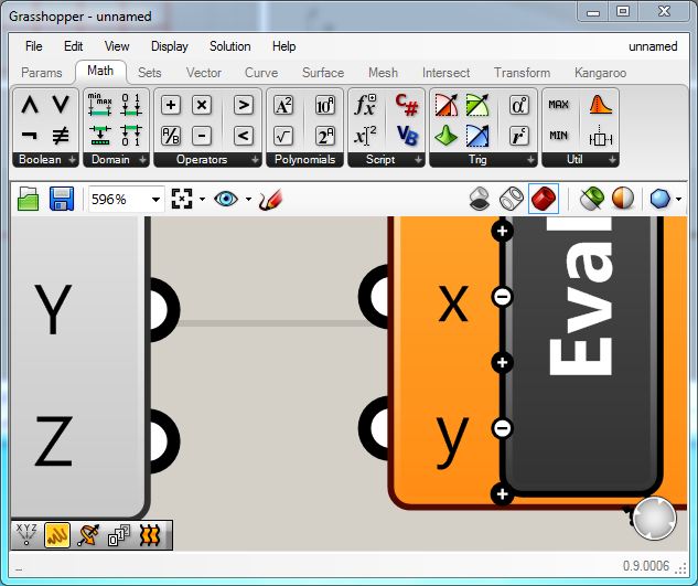
Within the Grasshopper window, zoom up on the function component, select the lower "+" maker to insert a new input parameter:
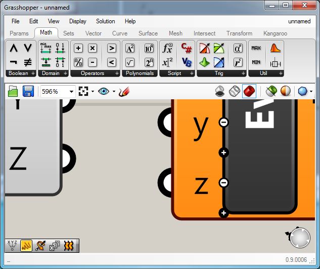
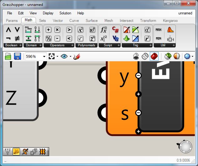
However, right-click on the letter "z' and change it to letter "s" so that it is more easily identified with the scalar coeficient "s":
Next, connect "Coeficient S" output port to the function input parameter "S", and the "x" and "y" parameters of the "Decompose" point component to the corresponding function input parameters "x" and "y". Save the Grasshopper File to "hyperbolicParabolicSurface.gh".
To complete the description of the function, right-click on the text "eval" and add the following expression.
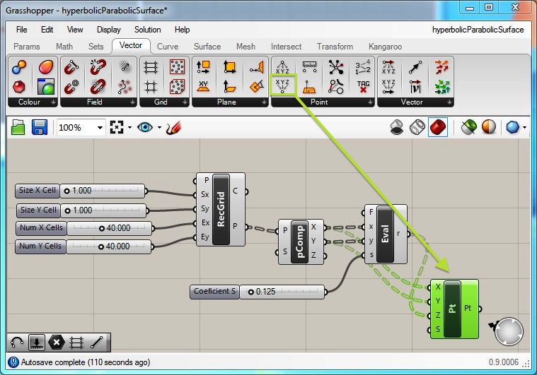
Next, go to the "Vector" tab and in the "Point" area select the "Point XYZ" component and place it in the Grasshopper work window to the lower- right of the function component. Connect the "x" and "y" output parameters of the "Decompose" point component to the corresponding input parameters "x and "y" of the new "Point XYZ" component, and connect the "r' output parameter of the hyperbolic parabolic function to tine input parameter "z" of the new "Point XYZ" component.
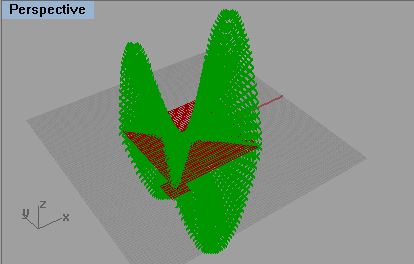
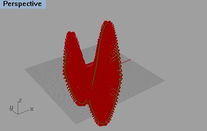
The last step resulted in Hyperbolic Parabolic grid points being displayed within Rhino.
Step 4: Create polygon mesh from the set of points.
In this final step, a surface is created from the hyperbolic parabolic set of points. Go to the "Surface" tab and in the "Freeform" area select the "Surface From Points" component and place it in the Grasshopper work window to the upper- right of the "Point XYZ" component. Connect the "Pt" output parameters of the point component to the corresponding input parameter "P" of the new "Surface From Points" component. Further more, right-click on "Pt" and select the option to "flatten" the output data. When the data is flattened, a down arrow appears on the right side of the data.
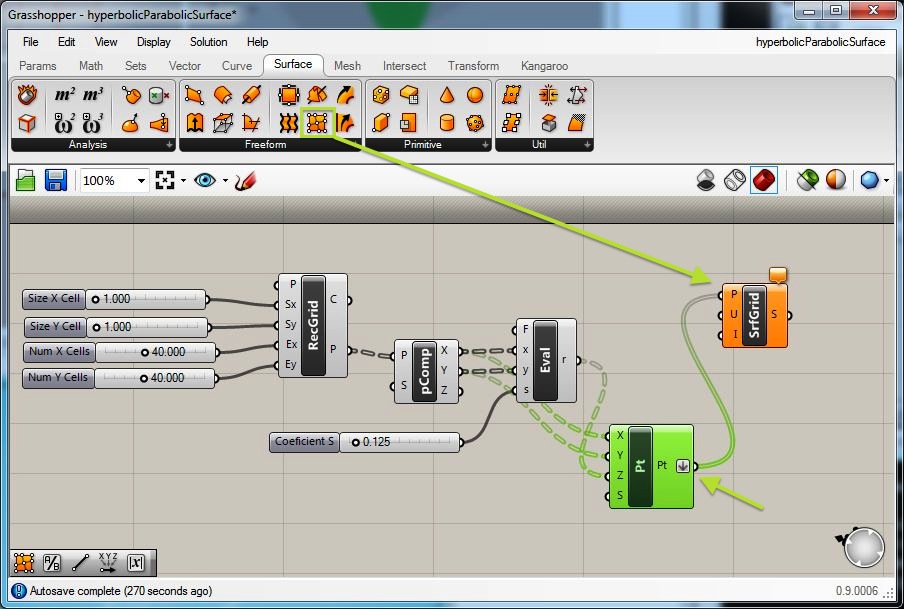
There
are still a few
more steps needed to specify the surface.
First, note that the internal coordinate system of control points for a
surface can be specified in terms of "U" and "V" parameters.
Furthermore, the number of points along the "U" edge of the
new
surface is equal to 1 plust the number of X cells specified
in
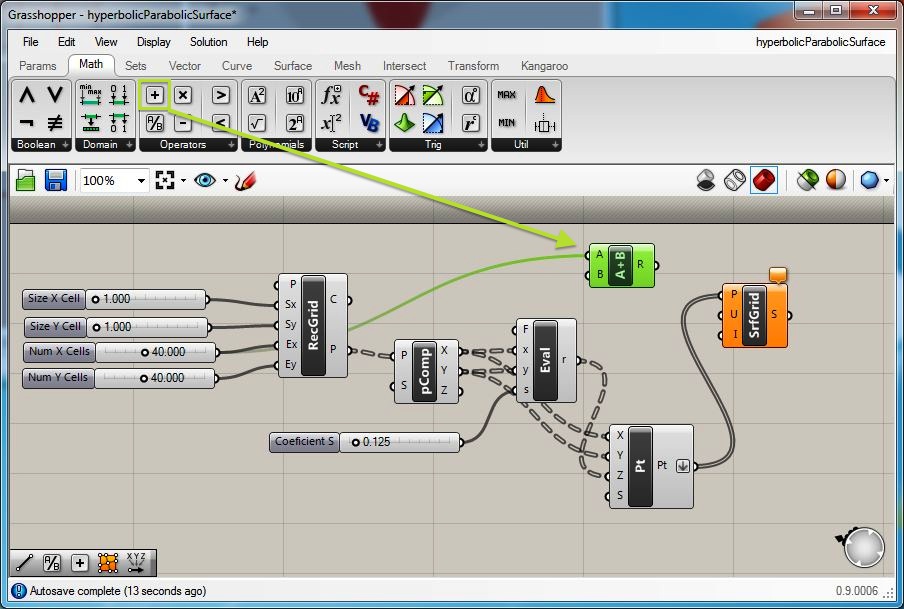
the "Num X Cell's" slider. Therefore,go to the
"Math" tab and in
the
"area" area select the "+" component and place it in the
Grasshopper work window to the upper- left of the "Surface
from
Points" component. Right-click on the the letter "B" of the "+"
component and set the value of the data item to "1'.
Also,
connect the output port of the "Num X Cells" slider to the input port
"A" of the "+" component.
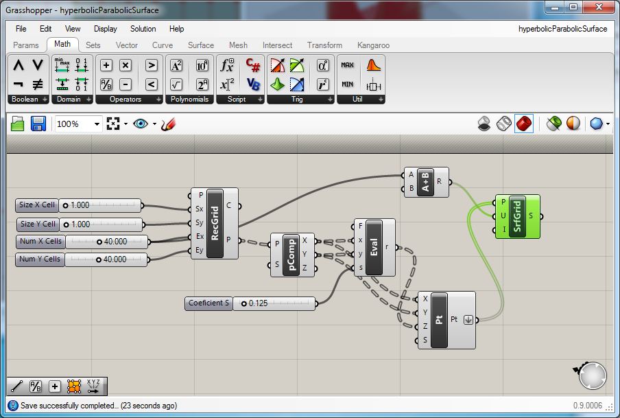
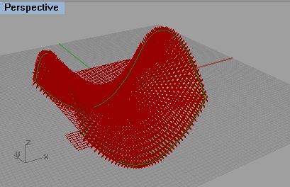
Finally, connect the "R" output parameter of the"+" component to the corresponding input parameter "U" of the new "Surface From Points" component, and the surface is generated.
Note that you can now modify the value for the
scalar
"Coeficient S" to adjust the vertical scale of the surface. Try for
example adjusting the value to 0.04 and see how the surface
is
modified.
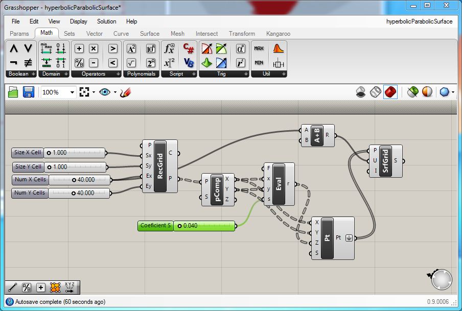
The height is lowered of the resulting hyperbolic parabolic surface.
 |
 |
| Coeficient S = 0.125 | Coeficient S
= 0.04 |
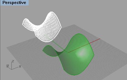
Step 5. Cleaning up the display.
Note that the display of graphics in Rhino that have been generated through Grasshopper are temporary by default. To turn off the display of any any graphic component, right-click on he component and toggle off the preview mode. On the other hand, to more permanently place a Grasshopper temporary element into Rhino, right-click on the related component and toggle on the "bake" mode. When toggling off all preview modes except for the final surface and then baking it into Rhino, we only see the original first point, the temporary surface (green) and then the baked surface (white) inside of Rhino. Note that the baked surface below was relocated with the "move" tool inside Rhino.
Note that if the value of coeficient "s" is lowered than the height of the resulting hyperbolic parabolic surface is also lowered.
Step 5. Other polynomial expressions.
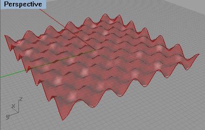
Using the same Grasshopper file, it is possible to generate other types of surfaces by using different algebraic expressions inside the eval function. Here are some possible alternatives and their results by using different algebraic expressions. Note that the coeficient scalar "S" has also been adjusted in these cases.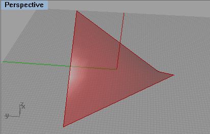 |
 |
 |
|
| Simple Saddle | Sine Surface | Eliptical Parabolic Surface | |
| s * (x * y) | s * sin (rad(x * 50)) * sin (rad(y * 50)) | -1 * s * (x² + y²) |
Some useful sites:
http://www.grasshopper3d.com/group/rhinopython
wiki.mcneel.com/developer/python
http://wiki.mcneel.com/developer/python
http://formecomplexe.files.wordpress.com/2012/04/grasshopper-tutorial.pdf
http://digitaltoolbox.info/grasshopper-basic/
http://blogs.cornell.edu/adaptivesystems/6_tutorial-3/
http://wiki.mcneel.com/developer/dotnetplugins
http://quicksilver.be.washington.edu/courses/arch486x/5.Grasshopper/6.Scripting/1.Introduction.html
http://theprovingground.wikidot.com/scripts-mathform
http://community.nus.edu.sg/DigitalDesignMedia/index.php/scripts/grasshopper-script/
http://wiki.mcneel.com/labs/grasshoppergallery