1. Creating Terrain File Using Geopak
-
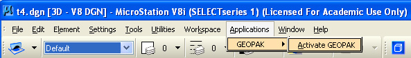
Geopak is loaded into Microstation by choosing Activate BENTLEY CIVIL under the Applications menu if not already done previously.
-
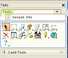
The task menus on the left-hand side of the Microstation window will now include a tab for "Geopak Site". Selecting this tab activates the set of menus that most directly relate to the use of Geopak.
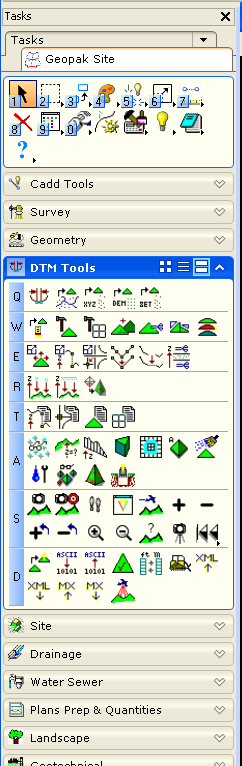
- Note that the prior set of menus can
be
restored by selecting the "Tasks" tab (highlighted in green
below) that is located just above the "Geopak Site" tab:
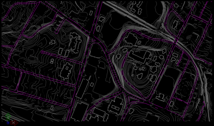
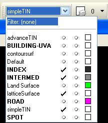
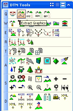
- Turn off the layer simpleDTM, and rotate into the top view such that only the contour lines are display (layers INTERMED and INDEX). Make advancedTIN the active layer
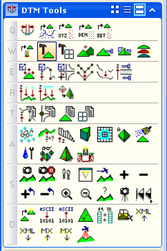
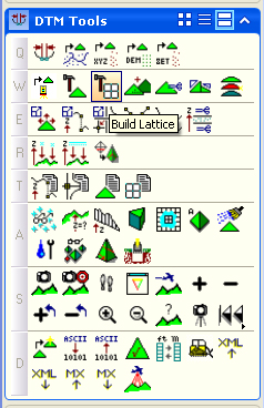
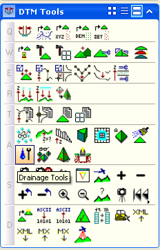
- From the DTM Tools
Tab, Select the "Extract Graphics" tool (Q2):
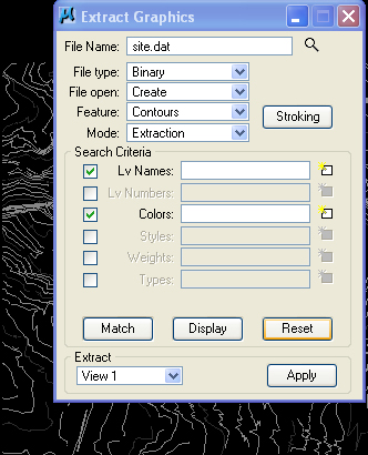
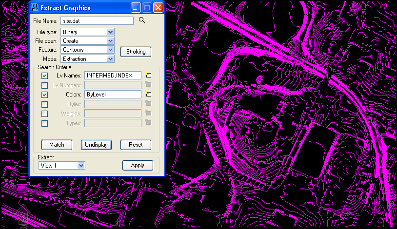
- The dialog box settings, set
File Type
to "Binary", File Open to "Create", Feature to "Contours", Mode to
"Extraction", and then under Search Criterion, check-on the check boxes
for Lv Names: and Colors, and hit the Reset button so that
all
the text fields for the search criterion are empty. Use the magnifying
glass icon in the upper right hand corner to name a new extraction file
such as "site.dat".
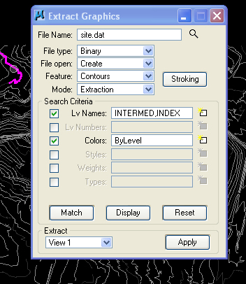
- Select "Match" button, and using the
left
mouse button, select one of the topo lines (eg., light gray). Accept
the selection by moving the mouse off the topo lines and hitting the
left mouse button once again in a area of the drawing without other
graphic elements. Repeat the same process for the second set of topo
lines (dark gray). The Extraction Graphics dialog box will then be
populated with the levels and colors of these two topo lines as follows:
- Select the "Display" button
and the
full set of elements founds by the Search Criteria will highly in Pink.
The name of the "Display" button will change to "Undisplay".
- Select the "Undisplay" button to turn
off
the highlight on the contours and select the "Apply" button to create
the external site.dat file.
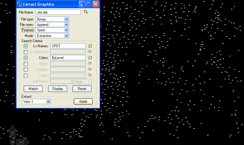
- The same file also contains
spot
elevation data. Turn on the the level named "SPOT, turn off
the
contour levels, and reset File Open to "Append" and Feature to "
Spots". Reset the Search Criteria and then use the same Match
technique as before to select the spot elevation data.
- Select the Apply button to append the
site.dat file with the additional SPOT elevation data. Thus, the
external site.dat file now is encompassing both contour and spot
elevation data.
- The next step requires converting the
dat
file to
an external tin file (triangulated irregular network file).
Select the Build Triangles tool and specify the source file
"site.dat" and the new file "site.tin" and select the "Build Triangle"
button.
select Build Triangles tool 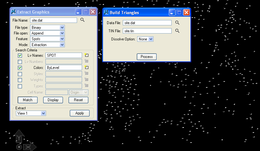
run Build Triangles tool to create site.tin file. - Similarly choose
the "Build
Lattice" tool (W3) to convert the site.tin file to
an
external site.lat file (a unform polygonal grid mesh file).
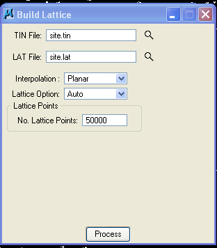
select Build Lattice tool run tool to convert site.tin to site.lat file
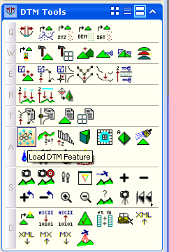
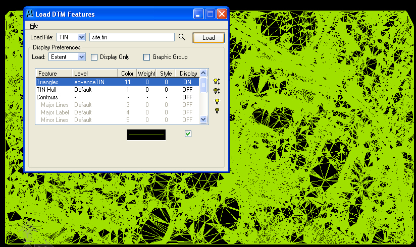
- The external files site.tin and
site.lat can
now be loaded back into Microstation. Here, choose the Load DTM
Feature tool (A1). In the load DTM dialog box,
set
Load File to "TIN", the file to load to "site.tin", turn on the
"Display Only" check-box, turn on the Triangles feature by
double-clicking on "Triangles" in the list of features. Then
double click on the horizontal graphic line below the features list to
launch the "Set Feature" dialog box, and designate Level as
"advanceTIN" and Color as 11.
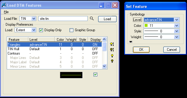
select Load DTM Feature tool set Tiangles feature type to load onto advanceTIN layer in color 11 - Select the "Load" button in
the Load
DTM Features tool to temporarily display the TIN model inside
Microstation. If this appears to be in good order, then turn off the
"Display Only" button and select the "Load" button again to more
permanently load the TIN model into Microstation.
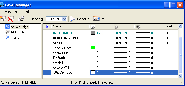
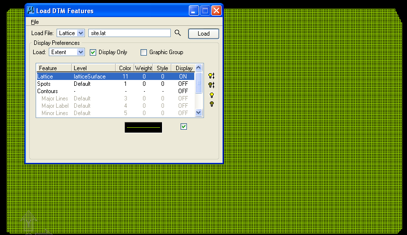
- Similary, in the Load DTM Features
dialog
box, the Lattice file can be loaded by changing the Load File type to
Lattice, selecting the file "site.lat", turning on the
lattice
feature "on", making "latticeSurface" the active level,
opening the "Set Feature"
dialog box, and
designating the Level as "latticeSurface" and the Color as
11.
This too can be tested with the "Display Only" option first
before loading the lattice file into Microstation.
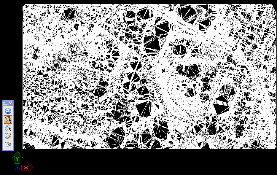
- Note that, using the same
method, the
"Contours" feature above can also be loaded into the model to
regenerate more normalized contours with major and minor interval lines
(see image under part 4, step 10 below).
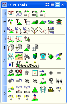
- Once these steps have been performed
inside
Geopak, a set of analytical tools is available to examine the features
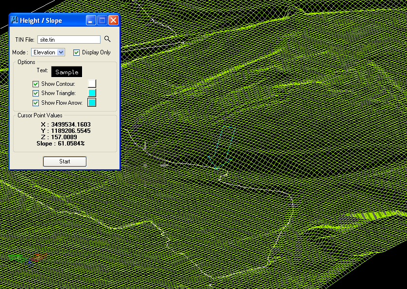
for such attributes as slope, drainage, etc. For example, the
"Height/Slope" tool (A2), can be selected to interactively explore the
hight slope of the terrain file. Note that you select the external file
"site.tin", turn on the check-boxes for showing contour lines,
triangles (TIN facets), and flow arrows, and select the "Start" button.
Moving the mouse over the drawing window will show slope (blue arrow
below), contour lines (white), and TIN triangle (blue), ans well as
echo back elevation and slope values numerically as depicted below.
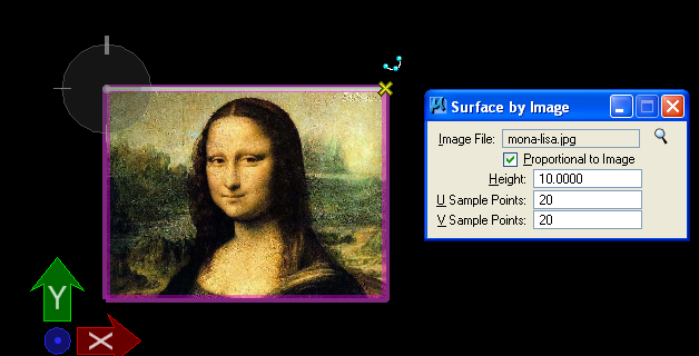
2. Terrain from Image File
- The Image
underlay file topo2.jpg that has been placed in in classes is a scanned
in image of a site plan with topological lines. –
- Note
the scale of topo2.jpg is
1”=300’ and the actual dimensions of the scanned
in image are 7.5 x 12
inches in paper size
- Close
the image
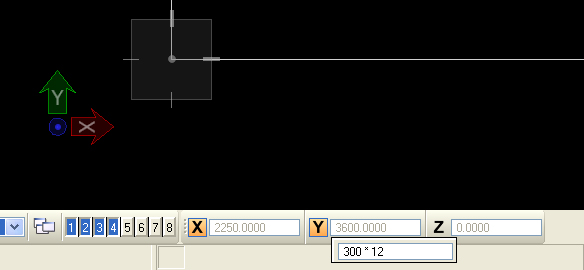
- Inside
Microstation, draw
rectangle at an appropriate size for attaching topographic
image
above, using the Addudraw popup calculator in the coordinate
text
boxes for "X" and "Y". After entering a lower left-hand data point,
then for the "X" coordinate enter "=" and then "300 * 7.5", and for the
"Y"coordinate enter "=" and then "300 * 12.0".
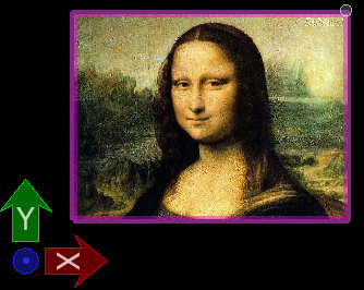
- Fit
View
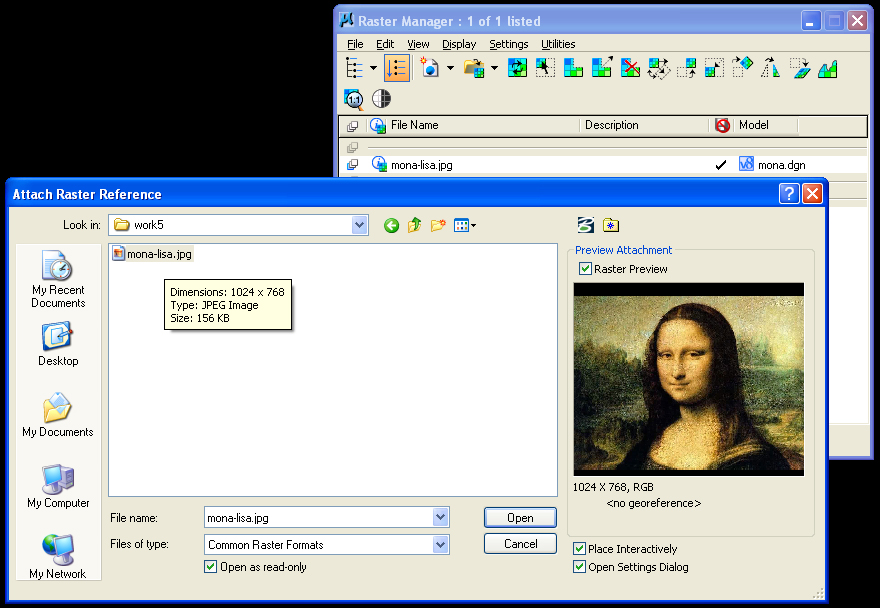
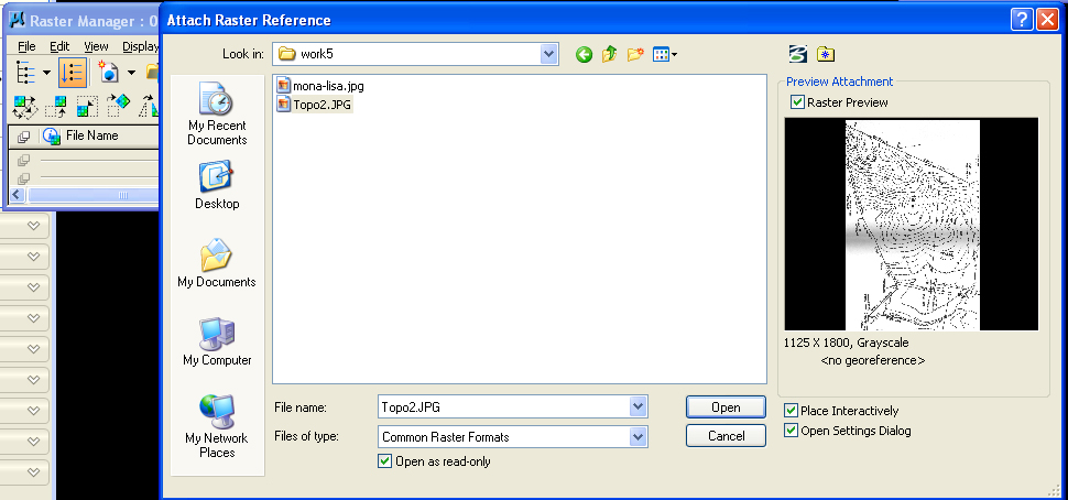
- Use
the File Menu/Raster Manager
dialog box, and interactively load the file topo2.jpg and use the
"Place Interactively" feature so that it is
scaled to the rectangle created in step 4.
- Use
the Utilities>KeyIn dialog
box, to enter "MDL
Load Civtools" (tool available for download
from School of Architecture file servers - see notes at beginning of this tutorial)
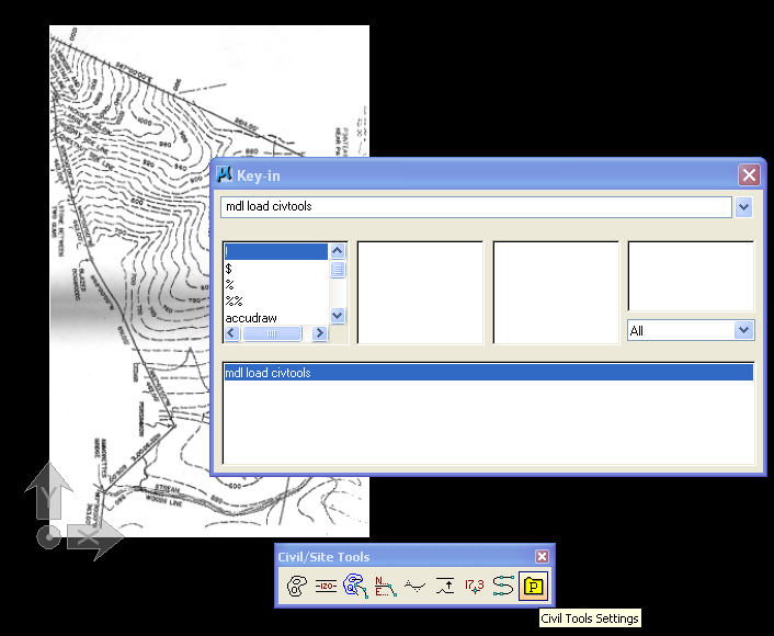
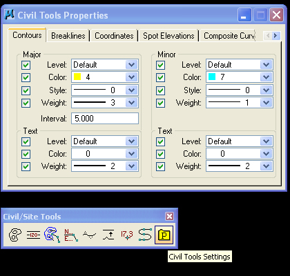
- Within the Civtools dialog box:
- [P]
tools – parameters – set
major/minor interval and colors/layers
- Choose
first tool – place contours - establish elevation level for
each
contour line and trace over the scanned in image using the curve tool
option, and setting "planar" check box to on.
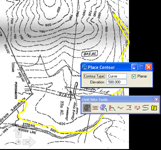
- Note:
you need to explicitly enter
in new elevation values into the Place Contour dialog box for each
contour line, such as the elevation 580' above.
- Set
current elevation – 600 – and draw
Keep going up the mountain.
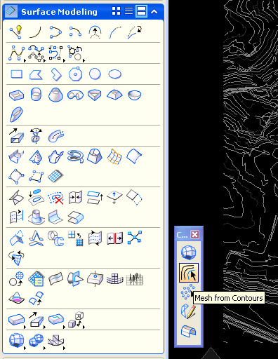
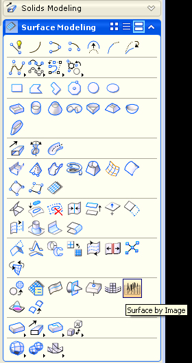
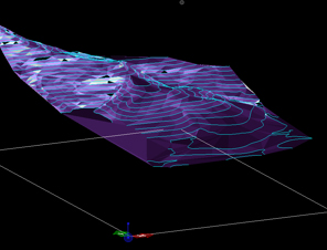
- Once the contours have
been
created, you may use either Surface tool "Mesh from Contours" tool or
the Geopak method to build a terrain file. (Here is a version
of
the above file with contour lines (blue) re-loaded and normalized from
the external TIN file.
- The greatest advantage
for
the Geopak method comes in the variety of analysis and modification
tools now available to explore the generated terrain model.
The Drainage tools allow you to see the flow of water on the surface. 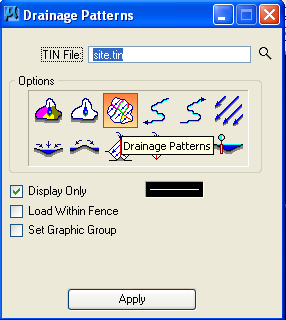
Drainage Patterns tool allows you to visualize the pattern of drainage as it applies to the entire surface. 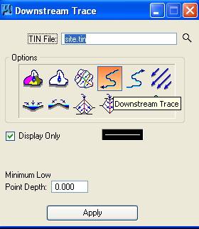
The Downstream Trace tpp; calculates the flow of water from a point (anywhere you click on the model) and will show it on the screen as a path. 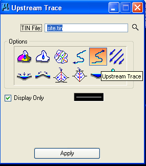
The Upstream trace allows you to trace a point (anywhere you click on the model) to where the source of water would be. 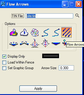
Flow Arrows show you the directinon o water flow accross the entire surface.
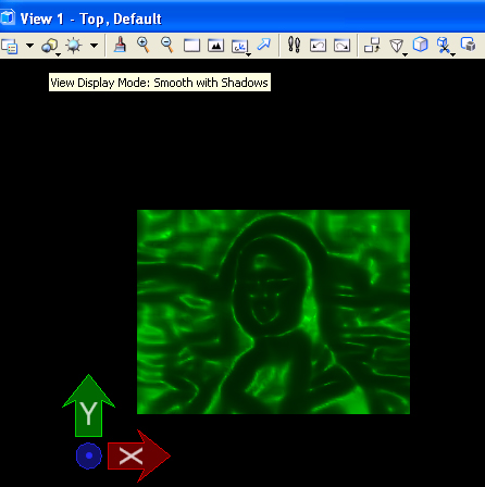
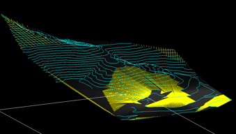
- The visibility tool gives
you line of site between selected
observation point and destination point, and
given thematic
colors for visible (yellow), not visible (dark gray). The image below
at right depicts the visible area in yellow from an observation
point to a target
point.
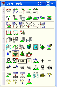
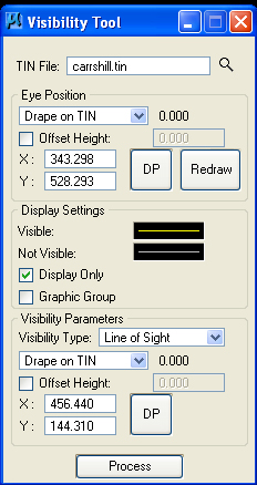
select Visibility Tool set display settings line of sight theme, visible (yellow), not visible (dark gray)
Additional thematic analysis tools available through Geopak provide for other types of slope, watershed and cut and fill analysis.
- Save the file to the Microstation dgn format. Open the dgn file direcly in Rhino. Within Rhino, re-save the file to the 3dm format. Note that Microstation can directly open a 3dm file, but can not save directly to the 3dm format. Simillary, Rhino can directly open a dgn file, but can not save directly to the dgn format.