
Computables of Architectural Design: Chapter 2
| For Internal UVa. Use Only: Funded by a Teaching and Technology Initiative Grant 1996 - 97 Draft: January 15, 1997 Copyright © 1997 by Earl Mark, University of Virginia, all rights reserved. Disclaimer |
Introducing The Graphic Coordinate System and Simple Graphics Programs
Our CAD system comes with predefined data types that may useful for creating geometry. We will explore these in some detail as we progress through the chapters of this text. These predefined data types allow us to build, access and modify geometry within a CAD drawing. They allow us to query the state of the drawing, and obtain other useful information. The system predefined data types are used similar to the manner of our own data type French-door of the previous chapter. We can assign and access their data via the dot "." operator. Within this chapter we will examine their use within the context of some simple graphics programs.
Three Dimensional Points
A predefined data type that is fundamental to the programming of the CAD system is a three dimensional point. The point is defined with with x, y, and z fields for each of its Cartesian coordinate locations. Within the Microstation CAD system, this point has been predefined this with the name of MbePoint. We can think of an MbePoint as having been predefined with the following expression:
|
The above expression lays out the fields for each of the Cartesian coordinate values of the point. That is, there is a field x declared as a double precision floating point number, y declared as a double precision floating point number, and z also declared as a double precision floating point number.
We have seen in the last chapter how to declare the variable door1, a specific case of the the use of our own predefined data type French-door. Similarly, here we can declare the variable StartPoint, a specific case of the system predefined data type MbePoint:
| Dim StartPoint As MbePoint |
Once the StartPoint has been declared, the individual fields within it might be assigned by means of the dot ". " operator as in the following example:
| StartPoint.x =1.0 StartPoint.y = 1.0 StartPoint.z = 0.0 |
A line segment within our CAD system could be described with both a StartPoint and an EndPoint. Accordingly, we might declare EndPoint as follows:
| Dim EndPoint As MbePoint |
Once the EndPoint has been declared, the individual fields within it might be assigned by means of the dot ". " operator as in the following example:
| EndPoint.x =2.0 EndPoint.y = 3.0 EndPoint.z = 0.0 |
Or, we might assign values to EndPoint using our earlier StartPoint as a reference as in the following example:
| EndPoint.x = StartPoint.x + 2 EndPoint.y = StartPoint.y + 2 EndPoint.z = StartPoint.z |
Note that for the sake of simplifying this discussion, we have not yet discussed the order of placement of the dim and the corresponding assignment statements within a computer graphics program. That is, we are only looking at fragments of the program but not how it is organized as a whole. The relative placement of BASIC statements within a program is a key topic that we turn to in the next section. A great part of how we generate and manipulate geometry within a CAD system is based on the use of predefined data types within simple graphics programs that we may write.
Writing A Procedure
In Chapter 1, we examined how to store data on the computer through the declaration of variables of different types (i.e., integer, real, and string). In the previous section, we looked at a predefined graphic data type. Now, we will explore how to use such data types within the context of a simple computer graphics program. A computer program may be referred to as a procedure. We might think of the term procedure in terms of its everyday use. A procedure is a sequence of instructions. A procedure has has been likened to a recipe for a cook. A procedure for making lasagna has both data and instructions.The data might consist of the raw ingredients (lasagna noodles, spinach,cottage cheese, parmesan cheese) and the instructions would consist of the steps (e.g., first lay down noodles, next lay down spinach, etc.) by which the raw ingredients are combined and baked.
Within the context of an architectural drawing, we might describe a procedure to guide someone through the steps of drawing a line starting at Cartesian Coordinate location (1,1) and extending 100 units to the right.. The architect Serlio hints at a general procedure for drawing a line in the Book of Architecture: "A line is a straight and continuous representation from one point to another, having length without width" [The Book of Architecture]. For our example of a line beginning at location (1,1), we might translate this description into the form of a short set of instructions:
| ' Locate the coordinates (1,1) of the
starting point of the line you wish to create ' Start drawing the line at (1,1) and proceed continuously ' Locate the coordinates (101,1) of the end point of the line you wish to create ' Stop drawing the line at (101,1) |
Within a CAD system such as Microstation, we might perform these instructions by hand by taking the following steps:
| ' Initiate the "place line" command ' Select point (1,1) on drawing screen with mouse and move mouse to the right continuously ' Select point (101,1) on the drawing screen with the mouse for the end point of the line ' Select the reset key to stop drawing the line |
Alternatively, we can write a procedure for the computer to automate these steps. The program below embeds several kinds of statements: (1) a non-executable comment line is preceded by a ' and is used repeatedly to tell us what the different parts of the program do. The comment line has no direct effect on what the program does, but only serves to document and clarify its processes to a person reading the text of program itself; (2) a variable declaration for point As MbePoint is incorporated into a Dim statement, (3) the main body of the program is signaled by the statement Sub main, (4)the end of the program is signaled by the statement End sub, (5) instructions are sent forth to the CAD system by statements of the form MbeSendxxxx. These MbeSendxxxx statements are then sequenced according to the steps required for the computer to draw the line, such as the statement MbeSendCommand "PLACE LINE " which invokes the CAD command to draw a line, or the statement MbeSendDataPoint point, 1% which sends point off to be used by the "PLACE LINE" command. We will become more familiar with these kinds of statements later in this chapter. First look at the program and its statements below, and then we will discuss its essential logic and order:
| 'A line is a straight and continuous representation
from one point to another, having length without width ' 'Place a line of 100 units starting at (1,1) Sub main ' Initialize and save space in memory for the information related to a Point Object Dim point As MbePoint ' Send the command that tells Microstation that you want to create a point on the window MbeSendCommand "PLACE LINE " ' Locate the coordinates of the starting point of the line you wish to create point.x = 1.0# point.y = 1.0# point.z = 0.0# ' Start drawing the line on window 1 MbeSendDataPoint point, 1% ' Locate the coordinates of the end point of the line you wish to create point.x = 100.0# point.y = 100.0# point.z = 0.0# ' Stop drawing the line on window 1 MbeSendDataPoint point, 1% ' Send a reset to the current command to stop placing points MbeSendReset End Sub |
The program includes the statement Dim point as MbePoint. This is really the graphics key to the entire work of the program. As we have seen before earlier in this chapter, any object dimensioned as an MbePoint includes an x, y, and z component. The assignment statements in the program such as point.x = 1.0# demonstrate how the Cartesian x, y, and z values are assigned to each point. Our program draws a diagonal line from point 1,1,0 to point 100,100,0 (see illustration below). You may note that the z-component of this lines' two endpoints is in both cases 0.0. The fact that the z-component is set to 0.0 means that the line is this is a two-dimensional line in the x-y plane. We will become more familiar with the CAD model space later.
If you have loaded this World Wide Web browser from within Microstation, you may run this program by selecting the following macro:
The Macro should produce a simple diagonal line from 1,1,0 to 100,100, 0 such as illustrated below:
|
Analysis of A Simple Graphics Program
The structure of the simple graphics program above applies to a great many others that we might develop for a CAD system. As we have seen in this example they consist of the following parts within an ordered sequence of steps:
The order is very important to the successful implementation of the program and its internal logic. In summary, we have established a process not unlike that of following a recipe: we use the MbeSendCommand statement to invoke the CAD command "PLACE LINE" to which we will send points; we establish the first endpoint; we MbeSendDataPoint the first endpoint to the "PLACE LINE" command; we establish the second endpoint; we MbeSendDataPoint the second endpoint to the "PLACE LINE" command; we use the MbeSendReset statement to conclude the use of the "PLACE LINE" command; finally, we use the End sub (end subroutine) statement to conclude the main body of the program.
Serlio's Description of Euclidean Geometry
Within Serlio's First Book On Geometry, a basic vocabulary of geometric elements serves to provide a foundation such that "the architect should be, if not learned in geometry, at least sufficiently knowledgeable so as to have some sort of understanding of it, particularly the general principles and also some of the more detailed matter. An abridged listing of these elements have been excerpted into the table below. Rather than provide a comprehensive introduction to Euclidean geometry, it was Serlio's intention to pick the "flowers" from Euclid that might provide an architect adequate knowledge to give a good account of whatever is built. [The Book of Architecture, translation by Hart & Hicks].
If you are reviewing this text on a World Wide Web browser that has been linked to Microstation, it is possible to use the table below more interactively. The Procedure column in the table contains a hypertext link to a Basic language program. If you select the procedure (e.g., Line ), then the figure will be automatically drawn in Microstation's active drawing window. The result will be comparable to the image at the far right. Each image at right in effect corresponds to a BASIC program. It also corresponds directly to Serlio's drawing in the The Book of Architecture. You may see the simple graphics program by selecting the Basic program link within the table below. Review these programs for their overall order of steps and internal logic. They each rely upon the predefined data type MbePoint as was discussed earlier in this chapter. They are simple but not necessarily efficient or written with great flair. Each contains more steps than really necessary to do the job at hand. They do not take advantage of certain techniques which we will explore later and which would greatly simplify the work and clarify the logic of what the programs do. They serve to introduce some more simple graphics programs of the type we had discussed in the previous section.
| Procedure | Description | Basic Program | Image |
| Point | First. a point is an indivisible thing, which has in itself no dimension. | Basic |  |
| Line | A line is a straight and continuous representation from one point to another, having length without width. | Basic |  |
| Parallel Lines | Parallels are two lines which continue at an equal distance. | Basic |  |
| Plane | A plane is made up of two equidistant lines closed off at the sides, that is a thing which has length and breadth without depth. It is also possible for planes to have different, unequal sides. | Basic |  |
| Equilateral Triangle | An equilateral triangle, that is of three equal sides, occurs when three lines equal in length are joined together. This figure will make three acute angles. | Basic |  |
| Right Triangle | A triangle of two equal sides occurs with two lines equal in length, that is one horizontal and the other perpendicular, and another longer line which forms the triangle. This will make one right angle and two acute angles. | Basic | 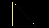 |
| Triangle of Three Unequal Sides | A triangle of three unequal sides occurs when three lines of unequal length are joined together. This figure will have three acute angles | Basic | 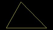 |
| Rectangle of Three Unequal Sides | A rectangle of unequal sides occurs with four lines of unequal length. This figure will have two obtuse angles. It could sometimes also have a right angle. | Basic | 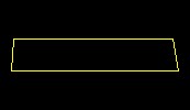 |
| Curvilinear bi-angular planes | Curvilinear bi-angular planes are made up of two curved, that is circular, lines. This shape will serve for many things in this book, and from it you can derive the correct normal, that is, the set square. The shape of the modern arches, which are called segmental arches, is taken from this form; and these arches can be seen upon many buildings on arched doorways and windows. | Basic | 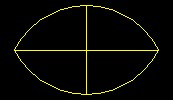 |
| Circle | The perfect circle has its centre, its circumference and its diameter. | Basic |  |
| Semi-circle | Semi-circle in which there is a plumb line falling upon the diameter. A right angle results from this, and it makes the half diameter. | Basic | 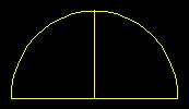 |
| Square | 'The perfect square occurs when four lines of equal length are joined together at right angles | Basic | 
|
Serlio relied upon these basic geometric constructions in the more advanced descriptions he employed. Similarly, we will embed these basic geometric figures into more advanced compositions in later chapters of this text. For now, it is important to take note of the direct correspondence between a graphic figure and the Basic procedure used to generate it. We are indebted to the early mathematicians, especially the Pythagorean, for seeing the correspondence between these parallel worlds. This link is critically important to the exploitation of computer aided design systems. We can setup parallel descriptions and work one against the other. That is, we use a Basic program to realize the creation of drawing. Conversely, and surprisingly, we can take a drawing and automatically convert it into a Basic program, at least at a fairly simple level. The following section describes how automatically build a Basic procedure from drawing.
Building A Program Prototype
Some CAD systems have the capacity to allow you to build a prototype of a program without actually typing in any code. This approach recognizes the notion that you are in effect programming a CAD system by hand when you undertake a series of drawing commands. In particular, we could have written the simple graphics program above without having to write the text directly. We could ask the CAD system to write the program for us while we draw the diagonal line. For example, we can have the series of steps recorded and then automatically translated into a program written in the BASIC language.This is a very convenient way to initialize the design of some computer graphics programs.
In this section, we briefly examine how build a BASIC program prototype through the automated technique. In Microstation, the BASIC program is also referred to as a macro. We will build the prototype of a macro by invoking the "PLACE LINE" command. Before starting the prototype session, you may need to configure your system to establish a search path so that your macro can be saved in your home directory on the computer or whatever other directory where you typically store your personal files. See your system manager if you are unfamiliar with this technique. If you are taking a course, this has likely been done for you. [Or, for those familiar with how to configure search pathways, this can be done within Mircostation by following a somewhat extensive set of instructions: (1) select the Configuration pulldown menu item from the Workspace menu within Microstation; (2) Select the Category for primary search paths; (3) go to the select default search paths for files sub-window and select Macros; (4) choose the select button; (5) in the dialog box which appears select the add button and locate the directory where you wish to store your work. For example, you might add the directory x:\mymacs for including a personal directory mymacs on the x drive.]
Once your personal Microstation configuration has been altered, enter the program and start a new drawing as instructed in the tutorials for the software (see end of chapter 1 for these instructions). Setup view windows and whatever other conditions you would presume be in effect before the Macro is invoked..That is, you may want to reproduce the kind of a situation where the MACRO would be run in the future. If doing this for the first time, a blank drawing is probably sufficient. In some situations, however, the MACRO might be created to operate on other pre-existing graphic elements. If the later case is true, then you might want to pre-establish the graphic elements to create the conditions where you begin to apply your macro.
Once you have completed the background preparations above,
start the macro generator by selecting the Create
Macro pulldown menu item from the Utilities menu within
Microstation. Save the macro to the designated directory
of your choice. A small tape recorder like icon will appear on
your screen with the play
button ![]() depressed to
indicate that the macro is recording. The name of the macro in
the example illustrated below is mymac and appears at
the the top of the recording tool window. Draw a diagonal line on
the screen with the PLACE LINE tool,
and then stop the recording
by pressing the last button (the black square)
depressed to
indicate that the macro is recording. The name of the macro in
the example illustrated below is mymac and appears at
the the top of the recording tool window. Draw a diagonal line on
the screen with the PLACE LINE tool,
and then stop the recording
by pressing the last button (the black square) ![]() to the right.
to the right.
 |
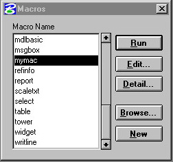
You are now well positioned to view the Macro and re-run it. Retrieve the macro program mymac by selecting the Macros pulldown menu item from the Utilities menu. A pop-up dialogue box will appear as illustrated below. This dialog box will contain a listing of any macros available in the default macro directory. Select the Browse button and move to the directory where your macro is located. In this example, load the macro mymac by highlighting it with the mouse and then selecting the Edit button.
 |
Selecting the Edit
button will bring up the macro in the BASIC program editor. Note
that there are several alternative ways of reviewing this
program. The right arrow button ![]() will play the program without stopping. To test the
program: (1) erase the original line segment that was used to
create the macro, and then (2) select the right arrow button
will play the program without stopping. To test the
program: (1) erase the original line segment that was used to
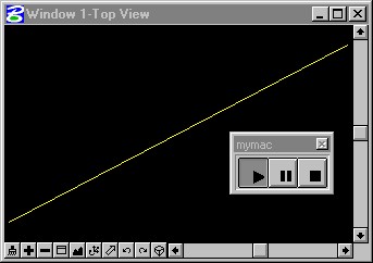
create the macro, and then (2) select the right arrow button ![]() and see the line segment
be redrawn. The line segment is drawn diagonally from the
location 0,0,0 to location 2,1,0 in exactly the same location as
the initial line segment.
and see the line segment
be redrawn. The line segment is drawn diagonally from the
location 0,0,0 to location 2,1,0 in exactly the same location as
the initial line segment.
 |
Modification of the program requires only that you move the mouse into the BASIC Editor window, and begin to edit the text. For example, you could change the program so that it draws a diagonal from the location 0,0,0 to 20,15,0 by making the changes to the values of the second datapoint as indicated below:
 |
Playing back the revised macro will result in a longer diagonal line drawn as follows.
 |
The debugger buttons located at the top of the macro window allow you to review and control the execution of the macro in greater detail..
Description of the macro control buttons:
The utility of some of these debugger buttons will become more apparent as we become familiar with more advanced aspects of the BASIC software language. The following table provides a summary level description of what the keys do.
| Button | Function |
| continue or initiate execution of the macro | |
| stop execution of the macro | |
| put a breakpoint in the macro | |
| execute one line of the macro; enter into any subroutine encountered | |
| execute one line of the macro; step over any subroutine encountered | |
| display variable values for viewing and modification |
Arithmetic Operations
Within the example programs of this chapter, we have used the + operator for addition. LISP has a representation for each of the other operators used in arithmetic expressions. These are summarized in the table below [from Microstation 95' BASIC reference]:
| Operator | Purpose | Number Arguments | Example | Result |
| + | addition of arguments | 2 | 1.4 + 2.0 | 3.4 |
| - | subtraction of arguments | 2 | 4.0 - 2.1 | 1.9 |
| - | negation of arguments | 1 | -5.0 | -5.0 |
| * | multiplication of arguments | 2 | 4.1 * 5.8 | 27.28 |
| / | Divide first argument by second argument | 2 | 24.9 /8.3 | 3.0 |
| \ | integer divide first argument by second argument | 2 | 5\3 | 1 |
| Mod | calculate integer remainder of first argument divided by second argument | 2 | 5 mod 2 | 1 |
| ^ | raise first argument to the exponent specified by the second argument | 2 | 3^2 | 9 |
The + operator is also may work on text strings, such as in the express "Archimedes "+"Spiral" which yields the concatenated expression "Archimedes Spiral". The & operator may used be used in the same way on two text expressions. Therefore, we have the string concatenation operators:
| Operator | Purpose | Number Arguments | Example | Result |
| + | concatenation of string arguments | 2 | "Archimedes " + "Spiral" | "Archimedes Spiral" |
| & | concatenation of string arguments | 2 | "Big Archimedes "& "Spiral" | "Big Archimedes Spiral" |
Several operators may be combined within a single expression. For example the expression 4 + 3 * 5 combines the addition and multiplication operators. When this is written into a BASIC program, the interpretation is not the same as it would be in standard algebraic interpretation. In particular, if we were to evaluate 4 + 3 * 5 in the standard way by hand, we would apply the operators from left to right. This expression would then be evaluated by first adding 4 to 3 to yield the number 7, and then multiplying the number 7 by 5 to yield the number 35. However, if the same expression of 4 + 3 * 5 were to be evaluated within a BASIC program, the order in which the operators are applied would be different. The computer's evaluation method would scan the expression from left to right as in the case of evaluating it by hand, but it would give precedence to some operators over other operators. That is, the evaluation still occurs from left to right, but operators with higher precedence are done first. In particular, it would give precedence to the multiplication operator * over the addition operator +. The evaluation would begin with the multiplication of 3 by 5 to yield the number 15, and then adding the number 4 to 15 to yield the number 19.
A few more expressions below give further evidence as to how the computer evaluation procedure works. Within each example, the initial line is replaced by a new line where the rules of evaluation have been applied in the correct order.
4 + 6 + 2 * 30
4 + 6 + 60 {multiplication operator is handled first
10 + 60 {result from adding 4 + 6
70 {result from adding 10 + 60
3 * 4 * 2 + 1
12 * 2 + 1 {result from multiplying 3 * 4
24 + 1 {result from multiplying 12 * 2
25 {result from adding 24 + 1
Note that parenthesis ( ) can be used to establish a precedence that overrides the normal operator precedence. We can apply parenthesis to the previous examples, and we change the results of the computer evaluations:
4 + (6 + 2) * 30
4 + 8 * 30 {parenthesis operator is handled first
4 + 240 {result of giving the multiplication operator precedence
244 {result adding 4 + 240
3 * (4 * 2 + 1)
3 * (8 + 1){result from multiplying 4 * 2
3 * 9 {result from adding 8 + 1
27 {result from multiplying 3 * 9
All the arithmetic operators have a precedence rating. Parenthesis can be used to override the precedence ratings and sometimes make expressions more understandable. The precedence ratings for the arithmetic operators from highest to lowest are listed in the following table [from Microstation 95' BASIC reference]:
| ( ) | Parenthesis |
| ^ | Exponentiation |
| - | Unary minus with one argument, e.g., -3 |
| *, / | Multiplication, Division |
| Mod | Modulo |
| +, - | Addition, Subtraction |
Summary
Within this chapter we have introduced the graphics Cartesian coordinate system and have illustrated some simple graphics procedures.We have also drawn a parallel between some basic graphics procedures and the Euclidean "flowers" which serve to lay out the basic geometry that Serlio finds relevant to describing architectural form. We noted that the process of doing a sequence of CAD commands by hand is similar to that of developing the steps within a simple graphics procedure. We further saw how a recording of the CAD commands done by hand can be translated into a prototype procedure. Finally, we reviewed the set of arithmetic operators and precedence rankings by which the arithmetic operators can be evaluated. As we develop more powerful procedures in the the following chapters, we will see how a these operators can be used to describe algebraically many geometrical forms found in nature and architecture. We will also see how the parenthesis operator can be used to give these algebraic expressions clarity and simplicity.
Within the next chapter, we begin to look at recurring relationships between similar kinds elements in a graphics composition. Some of these relations can be expressed concisely as a BASIC language procedure. The conciseness comes into play where we specify in just a few expressions a seemingly large number of recurring relations that occur in a graphics composition.
Homework 2: Prototype and Modify a Macro