Computables of Architectural Design: Chapter
7
| For Internal UVa. Use Only: Funded by a Teaching and Technology Initiative Grant 1996 - 97 Draft: January 15, 1997 Copyright © 1997 by Earl Mark, University of Virginia, all rights reserved. Disclaimer |
Introducing Three-Dimensional Geometry and Polynomial Surfaces
This chapter lays out some basic concepts and examples of three dimensional modeling. The foundation of these concepts begins with Euclid's theorem which states that three points determine a plane. We first use three points to develop a construction plane, and then we apply construction planes to generating computer based representations of three-dimensional geometry.
Descartes' development of Cartesian coordinates allowed problems in geometry to be reformulated into those in algebra (Ian Stewart,From Here to Infinity, Oxford University Press, 1996). We have already taken Descartes' important contribution for granted in the computer programs that rely upon two-dimensional coordinate geometry of the last chapters. However, we now develop some examples in three-dimensional space. We begin with simple rectangular polygons. We then use rectangular polygons to create surface elements.
Towards the end of this chapter, using Cartesian coordinates, we work out one of Serlio's three-dimensional examples and then expand upon it. This chapter also serves to introduce some the three-dimensional modeling concepts that underlie the case studies in the following chapters. Note that Serlio (1475 - 1554) preceded Descartes (1596 - 1650) by approximately one century, and so that this translation of Serlio's geometry into Cartesian coordinates is according to techniques not available in his time.
Construction Planes:
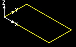
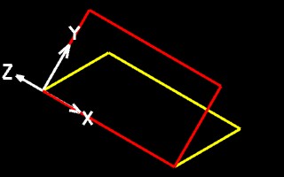
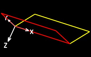
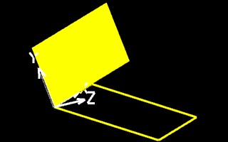
By convention, we can allow the three points to determine a specifically oriented Cartesian coordinate geometry where the first point determines the origin of a two-dimensional plane, the second point locates the x-axis and the third point gives the direction of the positive y-axis relative to the origin. The first figure below shows three such points identified in three-dimensional space. The second figure shows the positive x-axis and positive y-axis of a construction plane based on the initial three points. The third figure shows yet the direction of the positive z-axis relative to that construction plane.
| 3 Points Determine A Plane |
|
|
|
The direction of positive z is determined according to the right-hand rule. The right-hand rule is a convention that is related to the use of the right hand. That is: (1) place the base of your right hand thumb at the origin such that the tip of the thumb points in the direction of positive-x and (2) orient your right-hand such that its index finger (next to the thumb ) is pointed in the direction of positive-y, then (3) your right-hand middle finger bends 90 degrees forward towards your palm to determine the direction of positive-z.
Any number of arbitrary construction planes may be defined by three points. In the example below, each construction plane contains the geometry of an intersecting circle and square.
 |
A typical computer aided design system is based on the flexibility to describe three-dimensional geometry within any of these arbitrary construction planes. One such construction plane is designated as the Ground Construction Plane. It serves as the construction plane of basic reference and is typically co-planar with the ground plan of a three-dimensional model. Note that by convention, positive-y is pointed in the direction of North in the Ground Construction Plane, and by implication, negative-y is pointed in the direction of South, positive-x is pointed in the direction of East and negative-x is pointed in the direction of West. (Automated sun calculations are determined according to this convention, as can be adjusted to latitude, longitude and other factors).
 |
The World Coordinate System and The Local Coordinate System
The World Coordinate System of a three-dimensional computer aided design model is typically synonymous with the coordinate system determined by the Ground Construction Plane. That is, three-dimensional points specified relative to the Ground Construction Plane are given directly in the World Coordinate System point values. For example, we might specify a 2 x 1 dimensioned vertical rectangle in the x-z plane with four corner points specified in World Coordinates of (0.0, 0.0, 0.0), (2.0, 0.0, 0.0), (2.0, 0.0, 1.0), (0.0, 0.0, 1.0). In all prior chapters, we have been creating geometry by default in the Ground Construction Plane.
A Local Coordinate System refers to the coordinate system of any currently active construction plane. It may refer to the coordinate system of any of the arbitrary construction planes illustrated above. Or, it may also refer to the coordinate system of the Ground Construction Plane if it is presently active. In all prior chapters, we have been creating geometry by default in the Local Coordinate System of the Ground Construction Plane. In this chapter, we will also create geometry in alternative Local Coordinate Systems.
Three-Dimensional Specification Within A Computer Graphics Program
A three dimensional specification of geometry within a computer graphics procedure may be related to the x, y and z coordinate system of the Ground Construction Plane or of any of the arbitrary construction planes. For example, a line drawing in three-dimensional space may be specified in terms of its two end points (x1, y1, z1) and (x2, y2, and z2). Note that in chapter 2 we had predefined a data type MbePoint that may hold the coordinate information of any given point with the following expression:
|
The above expression lays out the fields for each of the Cartesian coordinate values of a three-dimensional point. That is, there is a field x declared as a double precision floating point number of the x-coordinate , a field y declared as a double precision floating point number of the y-coordinate, and a field z declared as a double precision floating point number of the z-coordinate of the three-dimensional point (review chapter 2 for more details).
Drawing A Polygon in the Local Coordinate System of the Ground Construction Plane: Trivial Case
The procedure that will be described below draws a Polygon in the Ground Construction Plane. It uses a particular CAD system set of conventions for explicitly activating the Ground Construction Plane. In this example program, the polygon is a simple 2 x 1 rectangle. When the procedure is modified further below, it draws a polygon in an alternative Local Coordinate System. Note that the white set of arrows is referred to as the Auxiliary Coordinate System icon and displays positive x, y, and z axis of the the currently active construction plane. The Auxiliary Coordinate System is synonymous with the currently active Local Coordinate System.
|
|
The procedure in the box below contains a few new features. It includes a point array called Points(), and it includes a technique for writing to a local coordinate systems. We first write our procedure to draw the rectangle in the left-hand figure above. We then modify the procedure to draw the tilted figure in the right-hand figure above.
Within the procedure, the array called Points() is used to hold the values of the points that define the rectangle. The elements of the array are indexed according to a zero based scheme, where the first point is identified by Points(0), the second point is identified by Points(1), and in general, the nth point is identified by Points(n - 1). The x-component of the first point is identified by Points(0).x, the y-component is identified by Points(0).y, and the z-component is identified by Points(0).z. Or, more generally, the x-component of the point n is identified by Points(n - 1).x, the y-component is identified by Points(n - 1).y, and the z-component is identified by Points(n - 1).z. Arrays of points are a convenient shorthand for storing the values of a number of points. We initially specify the dimension of the points() array with the statement Dim points() as MbePoint at the beginning of the Sub main procedure. When the procedure is running, we specify the actual size of the array with the statement redim points(numpts). In different language, we would say that the size of the points() array is initialized at runtime. Alternatively, we may have specified the size of the array with the statement Dim Points(4) as MbePoint. at the beginning of the Sub main procedure and would not have needed the use of the redim statement. The redim statement, however, is a convenient technique for handling the allocation of array sizes dynamically, and we shall see why this may be useful in later examples.
The sub procedure ChangeACS changes the currently active construction plane to that determined by three points of point1, point2, and point3, where point1 (0.0, 0.0, 0.0) locates he origin of the construction plane, point2 (1.0, 0.0, 0.0) locates the direction of the x-axis, and point3 (0.0, 0.0, 1.0) locates the direction of the y-axis. Within the sub-procedure ChangeACS, the points point1, point2, and point3 are submitted to the CAD system via the MbeSendDataPoint utility (i.e., MbeSendDataPoint point1). Use of the MbeSendDataPoint utility means by definition within Microstation that the points are submitted relative to the World Coordinate System. However, within the sub-procedure DrawPline below, the points point1, point2, and point3 are submitted to the CAD system via the SendAcsPoint procedure (i.e., SendAcsPoint(point1)).This involves the use of a particular Microstation command text keyin technique to draw in the active construction plane. In this example, the active construction plane happens coincidentally to be that of the World Coordinate System. The net effect is a trivial one. We could have drawn in the World Coordinate System directly with the use of the MbeSendDataPoint statement rather than using the SendAcsPoint procedure. However, we will soon use the SendAcsPoint procedure to draw in an alternative Local Coordinate System.
|
Procedure to draw a rectangle with the use of a local coordinate system, trivial case
Drawing A Polygon in alternative Local Coordinate Systems: Non-Trivial Cases
A modification to point3 in the sub main procedure changes the orientation of the local coordinate system to one that is tilted forward as represented by the ACS icon in the second of the two images above. That is, the change in the local coordinate system in turn causes the procedure to draw the red rectangle as depicted in the second image. The simple modification to point3 is as follows:
|
You may wish to test the variations the construction plane occasioned by the following assignments of values to points point1, point2, and point2, or experiment with other values..
|
|
Note that writing to a local coordinate system underscores the versatility of three-dimensional modeling techniques in computer aided design. In particular, a Local Coordinate System may help to simplify the description of drawing three-dimensional elements relative to other elements within a building or other three-dimensional object. For example, you might set the Local Coordinate System to be co-planar with the roof of a house, and then draw skylights and other elements relative to its geometry. Local Coordinate Systems are especially useful during development of a three-dimensional model where each command is input by the user manually through the available drawing tools one at a time rather than as facilitated by a computer graphics procedure. For the sake of simplicity in the next section, however, we develop descriptions of surfaces with respect to the World Coordinate System only. The techniques of using Local Coordinate Systems could be easily adapted to these surfaces so that they may be given any orientation in three-dimensional space.
Surface Descriptions
We first arrive at a surface description casually. The closed polygon sub procedure developed in the previous example can be modified to create a closed three-dimensional rectangular surface. In this next example, we rely upon the underlying display capability of a CAD system to convert the closed planar four sided polygon to a surface. That is, if we modify the procedure appropriately, then it will draw a rectangular surface rather than a wireframe rectangle. In the illustration below, a rectangular surface element sits at an incline relative to the wireframe rectangle. The points used to determine the Local Coordinate System are the same as those used in the last example. Note that within a typical CAD system, the surface elements are rendered visible by using a particular rendering tool. Within Microstation, the rendering tool is available under the utilities/render menu. It is possible to choose from the menu a variety of rendering algorithms each with its own special effect. The rendering below is achieved with the filled hidden line algorithm. For a further discussion of rendering techniques, see the appendix or refer directly to the CAD system rendering tutorials.
|
We need to modify our earlier procedure so that the polygons create a surface entity. In particular, the addition of a new sub-procedure CreateChain described in the box below will ensure that the polygons are closed entities and therefore that they create a surface. The procedure depends upon the technique of using a pointer (e.g., the variable fileposstart) that locates elements within the geometry database for the computer aided design system. The particular method of the sub procedure is specific to Microstation, but the general approach is applicable to other computer aided design systems. In order to apply this technique to any other given computer aided design system, it would be necessary to learn its specific conventions for marking positions in the geometry database.
Within the sub procedure DrawPoly, the end of the current drawing database is denoted with fileposstart. The variable fileposstart is a long integer that obtains its value from the expression fileposstart = MbeDgnInfo.EndOfFile. MbeDgnInfo is an object variable that contains information about the currently active drawing file, and EndOfFile is one of its components which holds the specific location of the end of that file. In the sub procedure DrawPoly, the variable fileposstart marks the end of the current drawing database. It also marks the location just before four lines are added with the PLACE LINE command. This means that the four lines are contained within the drawing database as the very next elements after the location of fileposstart. Finally, the sub procedure DrawPoly calls the sub procedure CreateChain to join all the lines in the current geometry file that are located after the marker fileposstart. To understand how CreateChain works in more detail, first review the code in the box below, and then read about the procedure CreateChain in the text that follows.
|
Sub procedure to draw a rectangle as a closed polygon surface
The sub procedure CreateChain employs a number of object variables. First these will be described individually, and then the sequence of the procedure will be summarized. The object variable element takes on information about graphics elements in the drawing file. The statement filepos = element.fromFile(fileposstart) is used to retrieve the location (filepos) of the first element in the drawing database that follows the location fileposstart. That is, it retrieves the location of the first line of the new polygon that has just been added to the geometry database. When the expression filepos = element.fromFile(fileposstart) assigns the value of -1 to filepos, then the end of the drawing database has been reached and there are no additional elements (i.e., polygon lines) to locate. Also appearing within the sub procedure, the command "CREATE SHAPE ICON" is used to link a number of elements together into a complex element. The statement MbeLocateElement filepos in effect tells the computer aided design system that the element located at filepos is to be identified and fed to the command "CREATE SHAPE ICON".
In summary, there are five basic steps to the sub-procedure CreateChain :
A Polynomial Surface
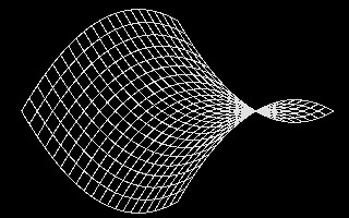
We have now established the basic foundation for developing a series of more advanced surface descriptions in three-dimensional space. In the examples below, polygons are described with reference to the World Coordinate System. This section picks out some polynomial expressions and the basic surfaces which they can produce. It is an eclectic collection derived from various textbook sources; however, there is consistency in how the basic surface elements are generated. In the examples given within this section, polynomial expressions are used to calculate the vertices of a number of simple four sided surface polygons. The four sided surface polygons are collectively arranged in three dimensional space so as to create larger surface areas. In the illustration below, we see a polygon wireframe description of a hyperbolic paraboloid shape on the left-hand side and its rendered surface description on the right-hand side [derived from Lord, The Mathematical Description of Shape and Form, John Wiley and Sons, 1984].
 |
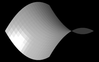 |
Hyperbolic Paraboloid in wireframe and surface renderings
The x-coordinate and y-coordinate of the polygon vertices range over a set of values stepping in increments of 1 from -10 to +10. That is, we have -10 <= Point.x <= 10 and -10 <= Point.y <= 10. Note that in the plan view below, the regularity of this uniform x-coordinate and y-coordinate grid mesh is apparent. However, the z-coordinate changes less uniformly from vertex to vertex and accounts most directly for the curvature that is apparent in the views of the surfaces above.
 |
 |
Plan View of Hyperbolic Paraboloid in Wireframe and Surface Renderings
The full BASIC program that generates the hyperbolic paraboloid surface will be given further below. First, however, we examine the logic of some of its parts. For each of the four sided polygons above, the z-coordinate value of each vertex is the function of its x-coordinate and y-coordinate values. The general mathematical expression used to calculate the z-coordinate of the vertices is:
|
where a, b and c are constants, z is the z-coordinate, x is the x-coordinate, and y is the y-coordinate value of a particular given polygon vertex in the figure above. Note that to generate the specific surface above, a = b = 1.0, c = 0.1, -10 <= x < 10, and -10 <= y <= 10. Modification of the constants a, b and c change the relative curvature of the surface, but not its basic canonical shape.
The polynomial is equivalently expressed within a BASIC program more directly in terms of each polygon vertex Point.x, Point.y, and Point.z as:
|
In particular, lets assume that we have a sub-procedure called SurfProc that takes a three dimensional Point and calculates its z coordinate Point.z based on the values of Point.x and Point.y according to the BASIC program expression above. The sub procedure SurfProc could be defined as indicated below.
|
Sub procedure that calculates the z-coordinate of the hyperbolic paraboloid surface
Now, to generate the surface, we need a way to organize every four adjacent vertices such that they form the individual polygons that constitute the overall surface. The following section of code contains two while loops that handle the work for some range of values in Point.x and Point.y. In the outer loop, MinX < Point.x < MaxX, where MinX = - 10, MaxX = 10 and the x-coordinate values of the adjacent four vertices of a polygon are incremented by 1.0 during each iteration. Within the inner loop, MinY < Point.Y < MaxY, where MinY = -10, MaxY = 10, and the y-coordinate values of the adjacent four vertices of a polygon are incremented by 1.0 during each iteration. Also within the inner loop, we calculate the z-coordinate value of each polygon vertex point with a call to the sub procedure SurfProc, and we draw each successive polygon with a call to the sub procedure DrawPoly. Note that the use of variables MinX, MaxX, MinY and MaxY provide a convenient place in the code to control the range of x and y coordinate values over which the surface is generated.In other words, we might increase the surface area by setting MinX = -20, MaxX = 20, MinY = -20, MaxY = 20 or some other such assignment that would extend beyond the range of -10 to 10 for the x-coordinate and y-coordinate values.
|
Fragment of sub procedure that processes four vertices of each polygon in 1 unit increments
The section of code we have generated thus far assumes that the x-coordinate and y-coordinate values of each point will increase in increments of 1.0, or, in other words, that each polygon is of a 1.0 x 1.0 dimension in the x - y plane. Alternatively, we could increase the resolution of the surface by reducing the increments to values of 0.5 so that each polygon is of a 0.5 x 0.5 dimension in the x - y plane.. Or more generally, we could use a variable called resolution so as to control the size of each polygon to a resolution x resolution dimension in the x - y plane as suggested in the following revised excerpt from the code.
|
Fragment of sub procedure that processes four vertices of each polygon in increments of the variable resolution
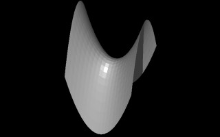
If we set the value of our resolution to 0.5, then the resulting surfaces appear as developed in the illustrations below. The smaller resolution value of 0.5 effects a smoother approximation of the hyperbolic paraboloid surface.
 |
 |
Hyperbolic Paraboloid in Wireframe and Surface Renderings at resolution of 0.5
Lets return again to the parameters controlling the generation of the hyperbolic paraboloid surface.We refer in the expression below to the initial statement that determines the value of z. It can be observed directly and straightforwardly that the constant c controls the scale of z. That is, if we double the value of the constant c, then we would correspondingly double the scale of the z-coordinates of the resulting surfaces.
|
The constant c acts as a scalar which we might isolate from the others by giving it the name Cscalar. The value of Point.z then is re-expressed within sub procedure SurfProc directly in terms of each polygon vertex Point as:
|
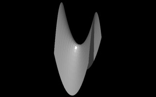
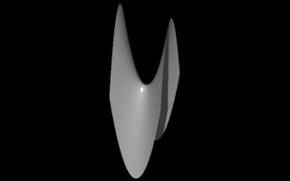
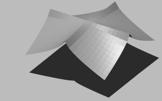
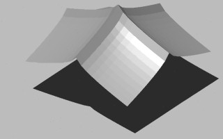
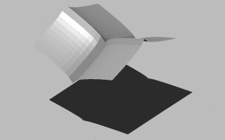
Within the following four illustrations, the value of Cscalar is increased in increments of 0.2. Each image has been re-scaled to fit the viewing frame (see the animation further below for relative scale). Reading the images from left to right and beginning with the first row, Cscalar values of 0.4, 0.6, 0.8 and 1.0 were used. Intuitively, it seems that the surface forms a kind of saddle. Since we form the hyperbolic paraboloid by squaring the values of x-coordinate and y-coordinate, we are not concerned with their positive or negative values, but rather with their distance from zero or, in other words, their absolute value. If the absolute value of the x-coordinate is high and the absolute value of y-coordinate is low, then the surface will rise up and the upper parts of the saddle are generated. If the absolute value of the x-coordinate is low and the absolute value of y-coordinate is high, then the surface will dip down and the lower parts of the saddle are generated. Middle range values for the x-coordinate and y-coordinate determine the middle levels of the saddle. Increasing the value of Cscalar accentuates the highs and lows of the surface form. Although not examined here for the sake of brevity, the impact of constants a and b might also be understood intuitively. If the absolute value of a < 1.0 and and the absolute value of b < 1.0, then it would have the impact of increasing the verticality of the surface as determined by the coordinates x and y respectively. Conversely, If the absolute value of a > 1.0 and and the absolute value of b> 1.0, then would have the impact of decreasing the verticality of the surface as determined by the coordinates x and y respectively.( Furthermore, since (Cscalar/2.0) is itself equal to a constant, we might substitute (Cscalar/2.0) with Cscalar thereby simplifying the equation slightly. However, if we retain the expression (Cscalar/2.0), then we find that setting the value of Cscalar to 0.1 often produce proportionately satisfying results, and the value of 0.1 seems to ground the expression in a useful way.)
 |
 |
 |
|
Cscalar values of 0.4, 0.6, 0.8 and 10.0.
The following animation depicts an increasing set of Cscalar values from 0.1 to 1.0. in increments of 1.0. Note that the surface changes in the z-axis only. Here, the scale of the images is maintained consistently so as to provide a relative size comparison of the different hyperbolic paraboloids.
 |
Animation of Cscalar values of 0.1 to 1.0 in increments of 1.0
As we will see in later examples, it is useful to further isolate the Cscalar parameter in generating a number of other surface types. We also find that in many cases that negating the value of Cscalar inverts the resulting surface which is generated. Therefore, it becomes useful to redefine the sub-procedure SurfProc with Cscalar as an input variable as indicated below.
|
Sub procedure that calculates z-values of a hyperbolic paraboloid surface
Note that we have now identified a number of key variables that will play a significant role in the fully constructed BASIC procedure. The variable resolution controls the scale of the individual polygons of the procedure. Smaller values for resolution provide for smoother surfaces. The variable Cscalar controls the scale of the z-coordinate of the surface polygons, thereby providing a means to control its overall vertical size. The variables MinX, MaxX, MinY and MaxY determine the range of x and y coordinate values over which the surface is generated.These variables and a few other techniques are now finally incorporated into the full procedure below that generates the hyperbolic paraboloid. Note also that to permit the code to run more quickly within Microstation, we have added the statements MbeSendCommand "NOECHO" and MbeSendCommand "ECHO" within sub Main . These statements turn off the text based readout of the embedded Microstation commands that would otherwise be echoed while the software is running.
|
Procedure to draw a hyperbolic paraboloid surface
Other Surfaces Formed By Polygons
Note that the modularity of this program permits the development of a number of other surface polygon procedures to be easily substituted for the hyperbolic paraboloid. These alternative surfaces may be generated by modifications only to the SurfProc procedure.
A upside-down elliptical paraboloid [Clapham] type of surface is generated by the following substitute for the SurfProc procedure. In particular, we have Point.z determined by the sum of the squares of Point.x and Point.y multiplied by Cscalar.
|
Sub procedure that calculates z-coordinate values of an elliptical paraboloid
If the absolute value of the x-coordinate is high and the absolute value of y-coordinate is high, then the surface will rise up and the upper parts of the dome are generated. If the absolute value of the x-coordinate is low and the absolute value of y-coordinate is low, then the surface will dip down and the lower parts of the surface are generated. The surface below is generated for a value of Cscalar as 0.1.
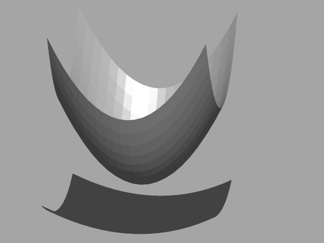 |
An "upside-down" elliptical paraboloid with Cscalar set to 1.0
If we negate the value of Cscalar to -1.0, then the following surface is generated.
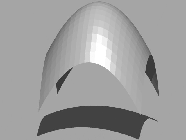 |
An elliptical paraboloid with Scalar set to -1.0
This behavior of Cscalar when isolated appropriately also has similar reversal effects on most of the examples that follow. From their mathematical definitions, we arrive at the generation of these additional surfaces through modification of the SurfProc procedure only. The remainder of the procedure is unchanged. In each case, we are simply substituting another polynomial expression in parameters Point.x and Point.y to arrive at a value for Point.z.
These case studies are now summarized in the following table:
Sub SurfProc (Point As MbePoint, Cscalar As Double) ' simple saddle[derived from Lord] Point.z = Cscalar * Point.x * Point.y end sub |
 |
Sub SurfProc (Point As MbePoint, Cscalar As Double) ' chair-like saddle[derived from Lord] ' most effective for low values of Cscalar such as 0.01 Point.z = Cscalar * Point.x^2 + Point.y^3 end sub |
 |
Sub SurfProc (Point As MbePoint, Cscalar As Double) ' single ridge surf[derived from Lord] ' Cscalar set to 0.1 Point.z = Cscalar * (Point.x)^2 - (abs (point.y))^0.667 end sub |
 |
Sub SurfProc (Point As MbePoint, Cscalar As Double) ' high peak double ridge surf [derived from Lord] ' Cscalar set to 0.5 Point.z = Cscalar * -1 * (abs (Point.x * Point.y))^0.667 end sub |
 |
Sub SurfProc (Point As MbePoint, Cscalar As Double) ' high peak double ridge surf [derived from Lord] ' Cscalar set to 1.0 Point.z = Cscalar *( -1 * (abs(Point.x))^0.6667 - (abs (Point.y))^0.6667) end sub |
 |
Sub SurfProc (Point As MbePoint, Cscalar As Double) ' dip and double ridge surface [derived from Lord] ' Cscalar set to -1.0, reverse effect of earlier case (two above) Point.z = Cscalar * -1 * (abs (Point.x * Point.y))^0.667 end sub |
 |
Sub SurfProc (Point As MbePoint, Cscalar As Double) ' sine wave in y ' Cscalar set to 1.0 with Resolution set to 0.5 Point.z = Cscalar * sin (Point.y) end sub |
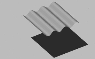 |
Sub SurfProc (Point As MbePoint, Cscalar As Double) ' sine wave in x and y ' Cscalar set to 1.0 with Resolution set to 0.5 Point.z = Cscalar * ( sin (Point.x) + sin (point.y)) end sub |
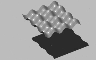 |
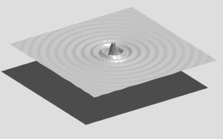
Sub SurfProc (Point As MbePoint, Cscalar As Double) ' concentric wave ' Cscalar set to 0.3 dim wavescl as Double, dist as Double wavescl = 0.75 dist = (sqr (point.x^2 + point.y^2)) Point.z = Cscalar * sin ((1.0 / wavescl) * dist) end sub |
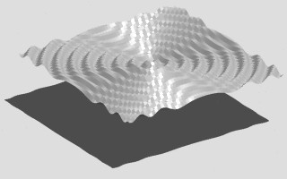 |
Sub SurfProc (Point As MbePoint, Cscalar As Double)
' concentric wave with attenuation - discontinuous procedure, Cscalar set to 3.0
  dim wavescl as Double, attenfac As Double, dist As Double
  wavescl = 0.75
  dist = (sqr (Point.x^2 + Point.y^2))
  if abs (dist) > 0.5 then
     attenfac = 2.0 / dist
  else
     attenfac = 1.0
  end if
  Point.z = Cscalar * attenfac * sin (1.0 / wavescl * dist)

end sub
|
 |
Sub SurfProc (Point As MbePoint, Cscalar As Double)
' peak - discontinuous function[derived from Lord]
  if (Point.x ^ 2 + Point.y ^2) >= 1 then
     Point.z = Cscalar * log (Point.x^2 + Point.y^2)
  else
     Point.z = Cscalar * log (1.0)
  end if

end sub
|
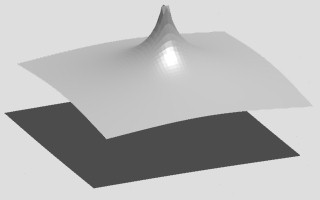 |
Note that the case of the concentric wave with attenuation in the example above involves the use of a a discontinuous function. That is, the variable dist is equal to the square root of the sum of the squares of point.x and point.y (i.e., dist = (sqr (Point.x^2 + Point.y^2)) ). If dist is equal to zero, then the expression attenfac = 2.0 / dist would involve division by zero. Therefore, for the sake of preserving the continuous shape of the wave, in all cases where dist < 0.5, we set atttenfac = 1.0. A similar use of a discontinuous function is used to control the shape of the peak in the next example, in this case to avoid calculating the log of 0.0.
Serlio's Simplified Description of Columns, Arches, and A Recessed Square
A more complicated application of surfacing technique may be adapted to Serlio's didactic example of a recessed square sitting upon arches and supported by columns. He develops this description for the purpose of teaching perspective rendering with the "the arches drawn simply so as to accommodate their bases and capitals" [Hart]. Serlio was primarily concerned with a simplification of geometry so as to facilitate a drawing lesson in perspective. We may also find within it a manner of succinctly approximating the geometry of a recognizable composition of classical elements. The columns lack the details of base, shaft and capital, but retain their essential proportions. Recall that Palladio's description of columns was introduced chapter 3 with a similar kind of simplicity of representation. The arches in Serlio's example are simple roman arches. The concise description lends itself well to replication within a computer procedure. As in our earlier case studies, we rely greatly upon four sided polygons in its description. We also add a few new kinds of elements.
 |
 |
 |
 |
Views of Serlio's Column, Arch, and Recessed Square Composition (Axonometric, Plan and Perspective Views)
We begin our analysis of the composition by first approximating the perspective orientation as that described by Serlio in Book II, plate 43v with some shadow details added.
 |
Here again we first examine the composition in its various parts before reviewing the computer graphics procedure as a whole. This code is necessarily complicated by two factors: (1) we are creating the above figure mainly with four sided polygon surfaces, which vary greatly in their geometry and spatial orientation, and (2) we interface with the somewhat idiosyncratic command syntax of a particular CAD system. These complications are not untypical of programming a CAD system and so our approach to this example is generally applicable to other architectural case studies that consist of a number of distinct shapes.
Lets examine the columns first. Within the drawing above, note that each column might be described as a tall box with truncated pyramid boxes of a base and capital. To begin our description of the column we develop the sub procedure excerpted below for a box. The box is centered at its base at CentrPt. It has dimensions for bottom box length BLen, bottom box width BWid, and also top box length TLen, top box width TWid, and box height VertDim. These dimensions are in turn used to calculate a rectangle consisting four points pointsbot() at the bottom of the box and four points pointstop() at the top of the box. Finally, the points pointsbot() and pointstop() determine the vertices of the six polygons that form the faces of the box. Each of the polygons is then drawn separately.
Note that the specification of the box permits the top face and lower face to have different dimensions. Therefore, the base of the column may be represented by a truncated pyramid type box with the bottom polygon face larger than the top polygon face. Conversely, the top of the column is represented by an upside-down truncated pyramid type box with the bottom polygon face smaller than the top polygon face.
  ''' M A K E   A   B O X   F R O M   S I X   F O U R   S I D E D   P O L Y G O N S
sub MakeBox (CenterPt As MbePoint, BLen As Double, BWid As Double, TLen As Double, TWid As Double, VertDim As Double)
    dim pointsbot(3) As MbePoint, pointstop(3) As MbePoint

'   Calculate corner points of base rectangle
    call CalcRect(CenterPt, BLen, BWid, Pointsbot())

'   Calculate corner points of top rectangle
    call CalcRect(CenterPt, TLen, TWid, Pointstop())
    Pointstop(0).z = CenterPt.z + VertDim
    Pointstop(1).z = CenterPt.z + VertDim
    Pointstop(2).z = CenterPt.z + VertDim
    Pointstop(3).z = CenterPt.z + VertDim

'   Draw Polygons for each side of box
    call DrawPoly (Pointsbot(0), Pointsbot(1), Pointsbot(2), Pointsbot(3))
    call DrawPoly (Pointsbot(0), Pointsbot(1), Pointstop(1), Pointstop(0))
    call DrawPoly (Pointsbot(1), Pointsbot(2), Pointstop(2), Pointstop(1))
    call DrawPoly (Pointsbot(2), Pointsbot(3), Pointstop(3), Pointstop(2))
    call DrawPoly (Pointsbot(3), Pointsbot(0), Pointstop(0), Pointstop(3))
    call DrawPoly (Pointstop(0), Pointstop(1), Pointstop(2), Pointstop(3))

    end Sub

''' C A L C U L A T E    R E C T A N G L E   P O I N T S
Sub CalcRect (Cpt As MbePoint, L As Double, W As Double, Pts() As MbePoint)
'   Calculate rectangle points based on center point, length and width
    Pts(0).x = Cpt.x - 0.5 * L
    Pts(0).y = Cpt.y - 0.5 * W
    Pts(0).z = Cpt.z
    Pts(1).x = Cpt.x - 0.5 * L
    Pts(1).y = Cpt.y + 0.5 * W
    Pts(1).z = Cpt.z
    Pts(2).x = Cpt.x + 0.5 * L
    Pts(2).y = Cpt.y + 0.5 * W
    Pts(2).z = Cpt.z
    Pts(3).x = Cpt.x + 0.5 * L
    Pts(3).y = Cpt.y - 0.5 * W
    Pts(3).z = Cpt.z

    End Sub
|
Sub procedures to make a box and calculate the vertices of a rectangle
The sub procedure MakeBox does much of the work of creating the Serlio composition. When appropriate dimensions are applied we are able to create boxes for all the forms of his composition with the exception of (1) the rectangles at the base, and (2) the arches and the walls directly above the arches. The rectangles of the base are straightforward and similar to the simple polygons we have created before. The explanation for them will be left to the code itself. However, in order to create the arches and the walls above the arches, a new technique is introduced in the code.
 |
 |
 |
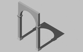 |
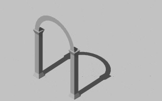
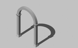
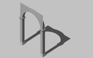
Generate arch profile and project arch [top row], generate wall above arch and project wall [ bottom row] (columns shown for reference)
The sub procedure DrawArch first traces out the profile of the arch in elevation (see above illustration). It begins with marking the end of the current database of the CAD drawing with the pointer fileposstart. The geometry of the arch is then calculated straightforwardly with respect to its center point CenterPt and radius ArchRadius, and also the distance between its introdos (inside arc) and extrados (outside arc) given as ColBaseDim. As indicated in the sub procedure, the extrados is drawn first, then the left-hand line which connects the extrados to the introdos, then the introdos, and then finally the right-hand line that connects the introdos to the extrados (see top left image in above table). The sub procedure CreateChain is then used to link these profile elements together. (Note that ColBaseDim is also the length of the side of the square plan of the column . This is important since the base of the arch, the distance between its intrados and the extrados, is this same dimension and therefore fits exactly on top of the square of the column.)
Once the arch profile has been created with the sub procedure CreateChain, it is projected horizontally using the sub procedure ProjElement (see top right image in above table). To understand how ProjElement works in more detail, first review the code in the box below, and then read the text that follows. The wall above the arch is created in a similar way of drawing its profile and then projecting it horizontally (see bottom row of images in the above table)
 ''' D R A W   A N   A R C H
sub DrawArch (CenterPt As MbePoint, ArchRadius As Double, ColBaseDim As Double)
'   Draw an arch
    dim Point1 As MbePoint, Point2 As MbePoint
    dim Point3 As MbePoint, Point4 As MbePoint
    dim fileposstart As Long, Vector As MbePoint

'   Mark the end of the current data base
    fileposstart = MbeDgnInfo.EndOfFile

'   Draw extrados of arch
    MbeSendCommand "PLACE ARC "
    point1.x = CenterPt.x + ArchRadius
    point1.y = CenterPt.y - (0.5 * ColBaseDim)
    point1.z = CenterPt.z
    MbeSendDataPoint Point1
    point2.x = CenterPt.x
    point2.y = CenterPt.y - (0.5 * ColBaseDim)
    point2.z = CenterPt.z + ArchRadius
    MbeSendDataPoint Point2
    point3.x = CenterPt.x -  ArchRadius
    point3.y = CenterPt.y - (0.5 * ColBaseDim)
    point3.z = CenterPt.z
    MbeSendDataPoint Point3
'   End Command By Sending Reset to Mouse
    MbeSendReset

'   Draw left-hand line at base of arch
    MbeSendCommand "PLACE LINE "
    MbeSendDataPoint Point3, 3%
    point3.x = point3.x + ColBaseDim
    MbeSendDataPoint Point3, 3%
'   End Command By Sending Reset to Mouse
    MbeSendReset

'   Draw intrados arch
    MbeSendCommand "PLACE ARC "
    point1.x = point1.x - ColBaseDim
    point2.z = point2.z - ColBaseDim
    MbeSendDataPoint Point1, 3%
    MbeSendDataPoint Point2, 3%
    MbeSendDataPoint Point3, 3%
'   End Command By Sending Reset to Mouse
    MbeSendReset

'   Draw right-hand line at base of arch
    MbeSendCommand "PLACE LINE "
    MbeSendDataPoint Point1, 3%
    point1.x = point1.x + ColBaseDim
    MbeSendDataPoint Point1, 3%
'   End Command By Sending Reset to Mouse
    MbeSendReset

'   Link graphic elements together
    call CreateChain (fileposstart)

'   Project arch according to plan thickness (ColBaseDim)
    vector.x = 0.0
    vector.y = ColBaseDim
    vector.z = 0.0
    call ProjElement (fileposstart, vector)

    End Sub

 ''' P R O J E C T   A N   E L E M E N T
sub ProjElement (fileposstart as Long, Vector as MbePoint)
'   Project element following fileposstart according to Vector
    dim Point as MbePoint, filepos as Long, element as New MbeElement

'   Pre-select elements to project
    MbeSendCommand "CHOOSE ELEMENT "
    filepos = element.fromFile(fileposstart)
    MbeLocateElement filepos

'   Start command construct element projection
    MbeSendCommand "CONSTRUCT SURFACE PROJECTION "

'   Set a variable associated with the dialog box to cap ends
    MbeSendCommand "ACTIVE CAPMODE ON "

'   Send two points forming projection vector
    Point.x = 0.0
    Point.y = 0.0
    Point.z = 0.0
    MbeSendDataPoint point
    Point.x = Point.x + Vector.x
    Point.y = Point.y + Vector.y
    Point.z = Point.z + Vector.z
    MbeSendDataPoint Point

'   End Command By Sending Reset to Mouse
    MbeSendReset

'   Deselect Element By Digitizing Empty Part of Drawing
    MbeSendCommand "CHOOSE ELEMENT "
    point.z = point.z + 1000
    MbeSendDataPoint point
    MbeSendReset

    End Sub
|
Sub procedures to draw an arch profile and project it horizontally
The sub procedure ProjElement takes the element identified from the drawing database by the pointer fileposstart and projects it according to the three-dimensional vector vector. The first step within the sub-procedure is to invoke the Microstation command "CHOOSE ELEMENT". This command is then fed the element at fileposstart. Note that the element is retrieved from the drawing database with the statement filepos = element.fromFile(fileposstart) similar to how this was done in the sub procedure CreateChain. In the case of creating the arch, the element at fileposstart is the arch profile. Through the technique of using the Microstation command "CHOOSE ELEMENT", the arch profile is in effect pre-selected for whatever Microstation command that follows. This is a standard technique of pre-selecting elements for one or more commands that may follow. In this case, the "CONSTRUCT SURFACE PROJECTION" command follows (see sub procedure ProjElement above). More specifically, the "CONSTRUCT SURFACE PROJECTION" command expects the pre-selected element of the arch profile and then requires description of two points that determine the magnitude and the direction intended projection. The projection vector is provided by two points which are calculated from the variable vector. Note that at the very end of the sub procedure ProjElement, we deselect the projected element by choosing an empty part of the drawing. This in effect is a safety measure to de-select the pre-selected elements and creates a kind of clean slate if a new Microstation command is invoked after the sub-procedure ProjElement is finished.
The remaining parts of the procedure to create the Serlio composition are based on the three techniques that we have now reviewed:
There are not any additional techniques needed to complete the drawing of Serlio's composition. All that is needed is the particular calculation of the geometry, the location and specific dimensions to the architectural elements. Therefore, these specific calculations are commented on directly in the code. Some while loops are incorporated to handle repetitions of columns, arches, etc.. The entire procedure appears now in the box below and is provided with comment lines in the code itself that explain its various parts.
 ''' D E C L A R E   S U B R O U T I N E S '''

    Declare Sub DrawBase (StartPoint As MbePoint,  ColBaseDim As Double, NumRows As Integer, NumCols As Integer, ColSpacing As Double)
    Declare sub DrawColumns (StartPoint As MbePoint, ColBaseDim As Double, NumRows As Integer, NumCols As Integer, ColSpacing As Double, CHeight As Double)
    Declare sub DrawArches (CenterPt As MbePoint, ArchRadius As Double, NumRows As Integer, NumCols As Integer, ColSpacing As Integer, ColBaseDim As Double, CHeight As Double)
    Declare sub DrawArch (CenterPt As MbePoint, ArchRadius As Double, ColBaseDim As Double)
    Declare sub DrawArchWall (CenterPt As MbePoint, ArchRadius As Double, ColBaseDim As Double)
    Declare sub CreateChain (fileposstart As Long)
    Declare sub DrawBeams (StartPoint As MbePoint, ArchRadius As Double, NumRows As Integer, NumCols As Integer, ColBaseDim As Double, CHeight As Double, ColSpacing As Double)
    Declare sub MakeBox (CenterPt As MbePoint, BLen As Double, BWid As Double, TLen As Double, TWid as Double, VertDim As Double)
    Declare sub DrawRect (CenterPt As MbePoint, Blength As Double, BWidth As Double)
    Declare sub CalcRect (Cpt As MbePoint, L As Double, W As Double, Pts() As MbePoint)
    Declare sub DrawPoly (Point1 As MbePoint, Point2 As MbePoint, Point3 As MbePoint, Point4 As MbePoint)
    Declare sub ProjElement (fileposstart as Long, Vector as MbePoint)

sub Main ()
    dim Numrows As Integer, Numcols As Integer, NumLevels As Integer, NumLevel As Integer
    dim ColBaseDim As double, ColSpacing As Double, CHeight As Double
    dim LHeight As Double
    dim StartPoint As MbePoint
    Dim ArchRadius As Double

    ColBaseDim = 1.0
    CHeight = ColBaseDim * 10.0
    NumRows = 2
    NumCols = 2
    NumLevels = 1
    ColSpacing = 10.0 * ColBaseDim
    ArchRadius = ColSpacing/2.0
    LHeight = CHeight + ArchRadius + ColBaseDim

'   Coordinates are in master units
    StartPoint.x = 0.0
    StartPoint.y = 0.0
    StartPoint.z = 0.0

    NumLevel = 1

    MbeSendCommand "NOECHO"

    while NumLevel <= NumLevels
        If NumLevel = 1 then
            call DrawBase (StartPoint, ColBaseDim, NumRows, NumCols, ColSpacing)
        End If
        call DrawColumns (StartPoint, ColBaseDim, NumRows, NumCols, ColSpacing, CHeight)
        call DrawArches (StartPoint, ArchRadius, NumRows, NumCols, ColSpacing, ColBaseDim, CHeight)
        call DrawBeams (StartPoint, ArchRadius, NumRows, NumCols, ColBaseDim, CHeight, ColSpacing)
        NumLevel = NumLevel + 1
        StartPoint.z = StartPoint.z + LHeight
    Wend

    MbeSendCommand "NOECHO"

    End Sub

''' D R A W   B A S E
Sub DrawBase (StartPoint As MbePoint,  ColBaseDim As Double, NumRows As Integer, NumCols As Integer, ColSpacing As Double)
'   Draw base of composition (first level only)
    dim CenterPt As MbePoint
    dim BLength As Double, BWidth As Double
    dim NumRow as Integer, NumCol as Integer
    dim BSpacing As Double

'   Draw Base Rectangle in Width (Plan Y-axis) Direction and Reset Spacing
    BLength = ColBaseDim
    BWidth = ColSpacing + (Colspacing - ColBaseDim) * (NumRows - 2.0)
    BSpacing = ColSpacing - 1.0
    CenterPt.x = StartPoint.x + 0.5 * BLength
    CenterPt.y = StartPoint.y + BWidth/2.0
    CenterPt.z = StartPoint.z
    NumCol = 1
    while NumCol <= NumCols
        Call DrawRect (CenterPt, BLength, BWidth)
        CenterPt.x = CenterPt.x + BSpacing * ColBaseDim
        NumCol = NumCol + 1
    wend

'   Draw Base Rectangle in Length (Plan X-axis) Direction and Reset Spacing
    BLength = ColSpacing + (Colspacing - ColBaseDim) * (NumCols - 2.0)
    BWidth =  ColBaseDim
    NumRow = 1
    CenterPt.x = StartPoint.x + BLength/2.0 'add
    CenterPt.y = StartPoint.y + 0.5 * BWidth
    CenterPt.z = StartPoint.z
    while NumRow <= NumRows
        Call DrawRect (CenterPt, BLength, BWidth)
        CenterPt.y = CenterPt.y + BSpacing * ColBaseDim
        NumRow = NumRow + 1
    wend

    End Sub

''' D R A W   T H E   C O L U M N S
sub DrawColumns (StartPoint As MbePoint, ColBaseDim As Double, NumRows As Integer, NumCols As Integer, ColSpacing As Double, CHeight As Double)
    Dim CentrPt As MbePoint
    Dim NumCol As Integer, NumRow As Integer
    Dim CapHeight As Double, CapVertDim As Double

'   Set dimensions of base and capital
    CapVertDim = 0.75 * ColBaseDim
    CapHeight = CHeight - CapVertDim

 '  Locate center of first column
    CentrPt.x = StartPoint.x + 0.5 * ColBaseDim
    CentrPt.y = StartPoint.y + 0.5 * ColBaseDim
    CentrPt.z = StartPoint.z
    NumRow = 1

'   Draw boxes for column shaft, base and capital, reset spacing, do next column
    while NumRow  <= NumRows
        NumRow = NumRow + 1
        NumCol = 1
        while NumCol <= NumCols
            call MakeBox (CentrPt, ColBaseDim, ColBaseDim, ColBaseDim, ColBaseDim, CHeight)
            call MakeBox (CentrPt, ColBaseDim * 1.5, ColBaseDim * 1.5, ColBaseDim, ColBaseDim, CapVertDim)
            CentrPt.z = CentrPt.z + CapHeight
            call MakeBox (CentrPt, ColBaseDim, ColBaseDim, ColBaseDim * 1.5,  ColBaseDim * 1.5, CapVertDim)
            CentrPt.z = StartPoint.z
            CentrPt.x = CentrPt.x + ((Colspacing - 1) * ColBaseDim)
            NumCol = NumCol + 1
        wend
        CentrPt.x = 0.5 * ColBaseDim
        CentrPt.y = CentrPt.y + ((Colspacing - 1) * ColBaseDim)
     wend

    End Sub

''' D R A W   T H E   A R C H E S
sub DrawArches (StartPoint As MbePoint, ArchRadius As Double, NumRows As Integer, NumCols As Integer, ColSpacing As Integer, ColBaseDim As Double, CHeight As Double)
'   Draw arches and walls directly above arches
    Dim CenterPt As MbePoint
    Dim NumRow As Integer, NumCol As Integer

    CenterPt.x = StartPoint.x + ArchRadius
    CenterPt.y = StartPoint.y + ColBaseDim/2.0
    CenterPt.z = StartPoint.z + CHeight
    NumCol = 2

'  Start drawing beginning with entire left-hand side of plan, and then moving to right
    While NumCol <= NumCols
        NumRow = 1
        while NumRow  <= NumRows
            call DrawArch (CenterPt, ArchRadius, ColBaseDim)
            CenterPt.y = CenterPt.y
            call DrawArchWall (CenterPt, ArchRadius, 0.8 * ColBaseDim)
            CenterPt.y = CenterPt.y + ((Colspacing - 1) * ColBaseDim)
            NumRow = NumRow + 1.0
        wend
        NumRow = 1
        NumCol = NumCol + 1
        CenterPt.y = StartPoint.y + ColBaseDim/2.0
        CenterPt.x = CenterPt.x + (Colspacing - 1) * ColBaseDim
    wend

    End Sub

''' D R A W   A N   A R C H
sub DrawArch (CenterPt As MbePoint, ArchRadius As Double, ColBaseDim As Double)
'   Draw an arch
    dim Point1 As MbePoint, Point2 As MbePoint
    dim Point3 As MbePoint, Point4 As MbePoint
    dim fileposstart As Long, Vector As MbePoint

'   Mark the end of the current data base
    fileposstart = MbeDgnInfo.EndOfFile

'   Draw extrados of arch
    MbeSendCommand "PLACE ARC "
    point1.x = CenterPt.x + ArchRadius
    point1.y = CenterPt.y - (0.5 * ColBaseDim)
    point1.z = CenterPt.z
    MbeSendDataPoint Point1
    point2.x = CenterPt.x
    point2.y = CenterPt.y - (0.5 * ColBaseDim)
    point2.z = CenterPt.z + ArchRadius
    MbeSendDataPoint Point2
    point3.x = CenterPt.x -  ArchRadius
    point3.y = CenterPt.y - (0.5 * ColBaseDim)
    point3.z = CenterPt.z
    MbeSendDataPoint Point3
'   End Command By Sending Reset to Mouse
    MbeSendReset

'   Draw left-hand line at base of arch
    MbeSendCommand "PLACE LINE "
    MbeSendDataPoint Point3, 3%
    point3.x = point3.x + ColBaseDim
    MbeSendDataPoint Point3, 3%
'   End Command By Sending Reset to Mouse
    MbeSendReset

'   Draw intrados arch
    MbeSendCommand "PLACE ARC "
    point1.x = point1.x - ColBaseDim
    point2.z = point2.z - ColBaseDim
    MbeSendDataPoint Point1, 3%
    MbeSendDataPoint Point2, 3%
    MbeSendDataPoint Point3, 3%
'   End Command By Sending Reset to Mouse
    MbeSendReset

'   Draw right-hand line at base of arch
    MbeSendCommand "PLACE LINE "
    MbeSendDataPoint Point1, 3%
    point1.x = point1.x + ColBaseDim
    MbeSendDataPoint Point1, 3%
'   End Command By Sending Reset to Mouse
    MbeSendReset

'   Link graphic elements together
    call CreateChain (fileposstart)

'   Project arch according to plan thickness (ColBaseDim)
    vector.x = 0.0
    vector.y = ColBaseDim
    vector.z = 0.0
    call ProjElement (fileposstart, vector)

    End Sub

''' D R A W   W A L L   A B O V E   A R C H
sub DrawArchWall (CenterPt As MbePoint, ArchRadius As Double, ColBaseDim As Double)
'   Draw Arch Wall
    dim point1 As MbePoint, point2 As MbePoint
    dim fileposstart As Long, filepos As Long
    dim element As New MbeElement, vector as MbePoint

'   Mark the end of the current data base
    fileposstart = MbeDgnInfo.EndOfFile

'   Draw extrados arc
    MbeSendCommand "PLACE ARC "
    point1.x = CenterPt.x + ArchRadius
    point1.y = CenterPt.y  - (0.5 * ColBaseDim)
    point1.z = CenterPt.z
    MbeSendDataPoint Point1
    point2.x = CenterPt.x
    point2.y = CenterPt.y  - (0.5 * ColBaseDim)
    point2.z = CenterPt.z + ArchRadius
    MbeSendDataPoint Point2
    point1.x = CenterPt.x -  ArchRadius
    MbeSendDataPoint Point1
'   End Command By Sending Reset to Mouse
    MbeSendReset

'   Draw lines on left, top and right-hand side relative to arch extrados
    MbeSendCommand "PLACE LINE "
    MbeSendDataPoint Point1, 3%
    point1.z = point1.z + ArchRadius * 1.1
    MbeSendDataPoint Point1, 3%
    point1.x = Point1.x + 2 * ArchRadius
    MbeSendDataPoint Point1, 3%
    point1.z = point1.z - ArchRadius * 1.1
    MbeSendTentPoint point1, 3%
    MbeSendDataPoint point1, 3%
'   End Command By Sending Reset to Mouse
    MbeSendReset

'   Link graphic elements together
    call CreateChain (fileposstart)

'   Project arch wall according to plan thickness
    vector.x = 0.0
    vector.y = ColBaseDim
    vector.z = 0.0
    call ProjElement (fileposstart, vector)

'   End Sub

end sub

''' C R E A T E   C H A I N   O F   L I N K E D   E L E M E N T S
Sub CreateChain (fileposstart As Long)
' Links together graphic elements in database from fileposstart to end of drawing database
    dim element As New MbeElement
    dim filepos As Long, fileposnew As Long

   filepos = element.fromFile(fileposstart)

'   Start a command
    MbeSendCommand "CREATE SHAPE ICON "
    do while filepos > -1
        MbeLocateElement filepos
        filepos = element.fromFile (filepos + element.filesize)
    loop

    MbeSendDataPoint 0,0,1000 'confirm union

    MbeSendReset

End Sub

''' D R A W   B E A M S
sub DrawBeams (StartPoint As MbePoint, ArchRadius As Double, NumRows As Integer, NumCols As Integer, ColBaseDim As Double, CHeight As Double, ColSpacing As Double)
    dim CenterPt As MbePoint
    dim BLength As Double, BWidth As Double, BHeight As Double
    dim BSpacing As Double, NumCol As Integer, NumRow As Integer

'   Draw beams in width (plan y-axis) direction and reset spacing
    BLength = ColBaseDim + 0.2 * ColBaseDim
    BWidth = ColSpacing + (Colspacing - ColBaseDim) * (NumRows - 2.0) + 0.2 * ColBaseDim
    BHeight = ColBaseDim
    Bspacing = ColSpacing - 1.0
    CenterPt.x = StartPoint.x + 0.5 * ColBaseDim
    CenterPt.y = StartPoint.y + BWidth/2.0
    CenterPt.z = StartPoint.z + ArchRadius + CHeight
    NumCol = 1

    while NumCol <= NumCols
        Call MakeBox (CenterPt, BLength, BWidth, BLength, BWidth, BHeight)
        CenterPt.x = CenterPt.x + BSpacing * ColBaseDim
        NumCol = NumCol + 1
    wend

'   Draw Beams in Length (Plan X-axis) Direction and Reset Spacing
    BLength = ColSpacing + (Colspacing - ColBaseDim) * (NumCols - 2.0) + 0.2 * ColBaseDim
    BWidth =  ColBaseDim + 0.2 * ColBaseDim
    CenterPt.x = StartPoint.x + BLength/2.0
    CenterPt.y = StartPoint.y + 0.5 * ColBaseDim
    CenterPt.z = StartPoint.z + ArchRadius + CHeight
    NumRow = 1

    while NumRow <= NumRows
        Call MakeBox (CenterPt, BLength, BWidth,  BLength, BWidth, BHeight)
        CenterPt.y = CenterPt.y + BSpacing * ColBaseDim
        NumRow = NumRow + 1
    wend

    End Sub

''' M A K E   A   B O X   F R O M   S I X   F O U R   S I D E D   P O L Y G O N S
sub MakeBox (CenterPt As MbePoint, BLen As Double, BWid As Double, TLen As Double, TWid As Double, VertDim As Double)
    dim pointsbot(3) As MbePoint, pointstop(3) As MbePoint

'   Calculate corner points of base rectangle
    call CalcRect(CenterPt, BLen, BWid, Pointsbot())

'   Calculate corner points of top rectangle
    call CalcRect(CenterPt, TLen, TWid, Pointstop())
    Pointstop(0).z = CenterPt.z + VertDim
    Pointstop(1).z = CenterPt.z + VertDim
    Pointstop(2).z = CenterPt.z + VertDim
    Pointstop(3).z = CenterPt.z + VertDim

'   Draw Polygons for each side of box
    call DrawPoly (Pointsbot(0), Pointsbot(1), Pointsbot(2), Pointsbot(3))
    call DrawPoly (Pointsbot(0), Pointsbot(1), Pointstop(1), Pointstop(0))
    call DrawPoly (Pointsbot(1), Pointsbot(2), Pointstop(2), Pointstop(1))
    call DrawPoly (Pointsbot(2), Pointsbot(3), Pointstop(3), Pointstop(2))
    call DrawPoly (Pointsbot(3), Pointsbot(0), Pointstop(0), Pointstop(3))
    call DrawPoly (Pointstop(0), Pointstop(1), Pointstop(2), Pointstop(3))

    end Sub

''' D R A W   A    R E C T A N G L E
Sub DrawRect (CenterPt As MbePoint, Blength As Double, BWidth As Double)
'   Draw rectangle of dimensions given
    dim Pts(3) As MbePoint

'   Calculate corner points of rectangle
    call CalcRect(CenterPt, Blength, BWidth, Pts())

'   Draw rectangle
    call DrawPoly (Pts(0), Pts(1), Pts(2), Pts(3))

    End Sub

''' C A L C U L A T E    R E C T A N G L E   P O I N T S
Sub CalcRect (Cpt As MbePoint, L As Double, W As Double, Pts() As MbePoint)
'   Calculate rectangle points based on center point, length and width
    Pts(0).x = Cpt.x - 0.5 * L
    Pts(0).y = Cpt.y - 0.5 * W
    Pts(0).z = Cpt.z
    Pts(1).x = Cpt.x - 0.5 * L
    Pts(1).y = Cpt.y + 0.5 * W
    Pts(1).z = Cpt.z
    Pts(2).x = Cpt.x + 0.5 * L
    Pts(2).y = Cpt.y + 0.5 * W
    Pts(2).z = Cpt.z
    Pts(3).x = Cpt.x + 0.5 * L
    Pts(3).y = Cpt.y - 0.5 * W
    Pts(3).z = Cpt.z

    End Sub

''' D R A W   A   P O L Y G O N   O F   F O U R   P O I N T S
sub DrawPoly (Point1 As MbePoint, Point2 As MbePoint, Point3 As MbePoint, Point4 As MbePoint)
'   Draw polygon of four points
    dim fileposstart As Long

'   Mark the end of the current data base
    fileposstart = MbeDgnInfo.EndOfFile

'   Draw lines
    MbeSendCommand "PLACE LINE "
    MbeSendDataPoint Point1, 3%
    MbeSendDataPoint Point2, 3%
    MbeSendDataPoint Point3, 3%
    MbeSendDataPoint Point4, 3%
    MbeSendDataPoint Point1, 3%

'   End Command By Sending Reset to Mouse
    MbeSendReset

'   Link lines together into single polygon
    call CreateChain (fileposstart)

    End Sub

''' P R O J E C T   A N   E L E M E N T
sub ProjElement (fileposstart as Long, Vector as MbePoint)
'   Project elements following  fileposstart according to Vector
    dim Point as MbePoint, filepos as Long, element as New MbeElement

'   Pre-select elements to project
    MbeSendCommand "CHOOSE ELEMENT "
    filepos = element.fromFile(fileposstart)
    MbeLocateElement filepos

'   Start command construct element projection
    MbeSendCommand "CONSTRUCT SURFACE PROJECTION "

'   Set a variable associated with the dialog box to cap ends
    MbeSendCommand "ACTIVE CAPMODE ON "

'   Send two points forming projection vector
    Point.x = 0.0
    Point.y = 0.0
    Point.z = 0.0
    MbeSendDataPoint point
    Point.x = Point.x + Vector.x
    Point.y = Point.y + Vector.y
    Point.z = Point.z + Vector.z
    MbeSendDataPoint Point

'   End Command By Sending Reset to Mouse
    MbeSendReset

'   Deselect Element By Digitizing Empty Part of Drawing
    MbeSendCommand "CHOOSE ELEMENT "
    point.z = point.z + 1000
    MbeSendDataPoint point
    MbeSendReset


    End Sub
|
Complete procedure to draw Serlio's recessed square sitting upon arches and supported by columns
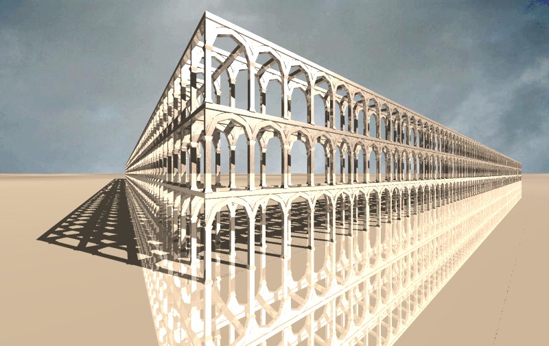
Finally, note that the sub main procedure of the code contains a number of key variables that control the dimensions and level of repetition in the composition. If NumRows = 2 and NumCols = 2 then we get a 2 x 2 array of columns, with each row of columns supporting an arch above it. We can begin to take liberties with the composition by setting NumRows = 3 and NumCols = 3, in which case we get 3 rows of columns and 6 arches. Furthermore, the variable BaseColDim is key to the entire scale of the composition. The scale can be doubled if we set BaseColDim = 2. Furthermore, we can begin to create several vertical levels of the composition if we set NumLevels = 3. Experimentation with the values to these variables will quickly yield a great range of possible repetitions of Serlio's initial composition. The image below represents one such variation where the program was run twice and a few rendering techniques added. In the first run NumCols = 100, NumRows = 2 and NumLevels = 30. In the second run NumCols = 2, NumRows = 100, and NumLevels = 3.
 |
Summary
Within this chapter we have developed a few basic techniques for representing three-dimensional surfaces . The principal building block of these surface elements has been a four side polygon. Initially we described how four sided polygons might be given any orientation in three-dimensional space as facilitated by the use of Local Coordinate Systems. We described how the lines within a four side polygon might be linked together to create a surface. We examined how such four side polygons could be arrayed together so as to create various kinds of polynomial and other surfaces. In our final example, we created a particular Serlio composition from four sided polygons that created boxes and also projected surface elements.
Our examples also demonstrates the power of encapsulating the basic parameters of a particular architectural composition within a few variables. In the case of polynomial related surfaces, we were able to succinctly describe the range of the surface (i.e., the variables MinX, MinY, MaxX, MaxY), the scale of its curvature (i.e., the variable Cscalar) and the resolution of its curvature (i.e., the variable resolution). In the case of Serlio's composition, we were able to control the basic scale (i.e., the variable ColBaseDim), and the degree of repetition of the basic elements (e.g., the variables NumCols, NumRows and NumLevels).
The encapsulation the variation in an architectural composition into a few basic parameters harnesses the power of the computer to respond most directly to a type of control that may most directly assert the thinking of a design about kinds of variation to be tested. This kind of encapsulation always runs the risk of oversimplification. For example, our last procedure would need to be modified to incorporate scale and orientation changes for Serlio's composition as we generate the different levels, rows and columns. This kind of is adjustment well within the concepts we have discussed and might be left as an exercise to the reader. More reflectively, however, we begin to assess here the computability of certain architectural forms, what is admitted within a straightforward computer graphics procedure, and what might be treated on an exceptional basis. This level of composition making begins to address the real difficulty and interest of architecture, where the order of the whole composition is not easily described within one comprehensive description. Yet, at some levels of representation and abstraction, we now have arrived at some some techniques for capturing the order of some aspect of design. These methods will grow in sophistication as we capture the order of some architectural forms in solid models in the chapters that follow.