COMPUTER
AIDED
ARCHITECTURAL DESIGN
Workshop 15 Notes,
Week of November 15 , 2015
SURFACES BASED UPON POLYNOMIAL EXPRESSIONS
This section picks out some polynomial expressions and the basic surfaces which they can produce.In the examples below, polygons are described with reference to the World Coordinate System. It is an eclectic collection derived from various textbook sources; however, there is consistency in how the basic surface elements are generated. In the examples polynomial expressions are used to calculate the vertices of a number of simple four sided surface polygons. The four sided surface polygons are juxtaposed in three dimensional space so as to create larger surface areas.
PART
1. Hyperbolic Parabolic Surface
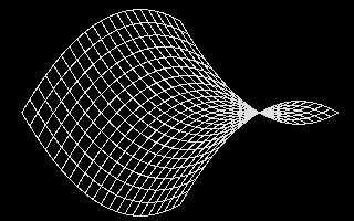
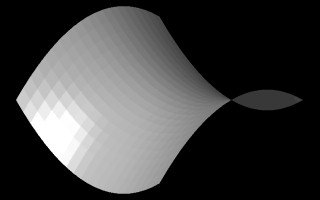
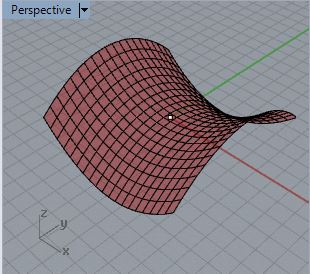
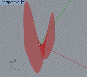
In the illustration below, we see a polygonal mesh description of a
hyperbolic paraboloid shape on the left-hand side and its rendered surface
description on the right-hand side [derived from Lord, The Mathematical
Description of Shape and Form, John Wiley and Sons, 1984].
|
|
Perspective View Hyperbolic Parabolic surface
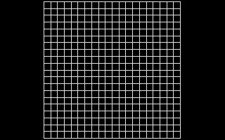
The x-coordinate and y-coordinate of the polygon vertices range over a
set of values stepping in increments of 1 from -10 to +10. That is, we
have -10 <= Point.X <= 10 and -10
<= Point.Y <= 10. Note the
regularity of this uniform x-coordinate and y-coordinate grid mesh is
apparent when seen in the plan view as depicted below. However, the
z-coordinate changes non-uniformly from vertex to vertex and accounts
most directly for the curvature that is apparent in the views of the
surfaces above.
 |
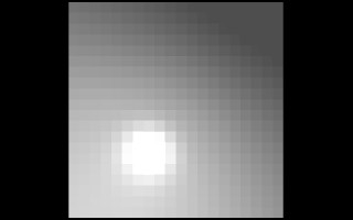 |
Plan
View Hyperbolic Parabolic surface
Sub procedure that calculates the
z-coordinate of the hyperbolic paraboloid surface
The full Python script that generates the hyperbolic paraboloid surface will be given further below. First, however, we examine the logic of some of its parts. For each of the four sided polygons above, the z-coordinate value of each vertex is the function of its x-coordinate and y-coordinate values. The general mathematical expression used to calculate the z-coordinate of the vertices is:
|
where s is a scalar coordinate, z is the z-coordinate, x is the x-coordinate, and y is the y-coordinate value of a particular given polygon vertex in the figure above, and where "pow" exponentiation function. Note that to generate the specific surface above, cScalar = 0.1, -10 <= x < 10, and -10 <= y <= 10. Modification of the scalar s impacts the relative height the z-coordinate each polygon vertex:
In particular, examine the function surfProc that takes a three dimensional Point and calculates its z coordinate Point.Z based on the values of Point.X and Point.Y and the scalar cScalar. That is, graphics function surfProc takes in x, y, and cScalar, and returns a new point named newPoint with the new z coordinate as indicated below.
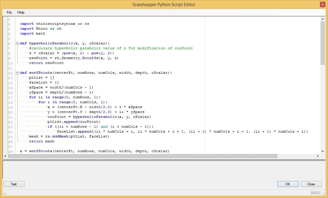
| def
hyperbolicParabolic(x, y, cScalar): ....#calculate hyperbolic parabolic value of z for modification of curPoint ....z = cScalar * (pow(x, 2) - pow(y, 2)) ....newPoint = rh.Geometry.Point3d(x, y, z) ....return newPoint |
PART
2: Calculating polygon grid faces of hyperbolic paraboloid
surface
In the following figure, there are nine vertices, labelled 0 through 8, and four associated faces determined by vertices (0, 1, 4, 3), (1, 2, 5, 4), (3, 4, 7, 6) and (4, 5, 8, 7). To generate the surface, we need a way to organize every four adjacent vertices such that they form the individual grid faces that constitute the overall surface. Thus a list of all the vertices and an indexing system that determines all the subgroups of 4 vertices forming each face are both needed. (This example is modified after a rhinoscriptsyntax help example provided by McNeel Inc.)
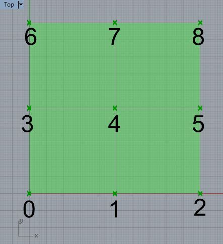
A python script to generate the polygon mesh surface and index into the vertices would be as follows. Note that the "faceVertices" array contains a list of index locations in the "vertices" array for each face of the polygon mesh.
| import
rhinoscriptsyntax as rs import Rhino as rh #vertices of polygon mesh pt0 = rh.Geometry.Point3d(0, 0, 0) pt1 = rh.Geometry.Point3d(5, 0, 0) pt2 = rh.Geometry.Point3d(10, 0, 0) pt3 = rh.Geometry.Point3d(0, 5, 0) pt4 = rh.Geometry.Point3d(5, 5, 0) pt5 = rh.Geometry.Point3d(10, 5, 0) pt6 = rh.Geometry.Point3d(0, 10, 0) pt7 = rh.Geometry.Point3d(5, 10, 0) pt8 = rh.Geometry.Point3d(10, 10, 0) #create array of vertices vertices = [pt0, pt1, pt2, pt3, pt4, pt5, pt6, pt7, pt8] #create index into vertices array to determine faces faceVertices = [] faceVertices.append((0,1,4,3)) faceVertices.append((1,2,5,4)) faceVertices.append((3,4,7,6)) faceVertices.append((4,5,8,7)) a = rs.AddMesh( vertices, faceVertices ) #output variable a b = vertices #output variable b |
Similarly, the following function contains two while loops that handle the work of creating faces for some range of values in Point.X and Point.Y. In the outer loop, -depth/2.0 <= Point.Y= <depth/2.0, and in the inner loop -width/2.0 <= Point.X <= width/2.0. Within the inner loop, we calculate the z-coordinate value of each polygon vertex point with a call to the sub procedure hyperbolicParabolic.
| def
makePolyMesh(centerPt, numRows, numCols, width, depth, cScalar): ....ptList = [] ....faceList = [] ....xSpace = width/(numCols - 1) ....ySpace = depth/(numRows - 1) ....for ii in range(0, numRows, 1): # outer loop handles values of y ........for i in range(0, numCols, 1): # inner loop handles values of x ............x = (centerPt.X - width/2.0) + i * xSpace ............y = (centerPt.Y - depth/2.0) + ii * ySpace ............curPoint = hyperbolicParabolic(x, y, cScalar) ............ptList.append(curPoint) # build the array of vertices ............if ((ii < numRows - 1) and (i < numCols - 1)): ............faceList.append((ii * numCols + i, ii * numCols + i + 1, (ii + 1) * numCols + i + 1, (ii + 1) * numCols + i)) # build index of faces corresponding to the array of vertices ....mesh = rs.AddMesh(ptList, faceList) ....return mesh |
Note that also build up an array consisting of sets of face vertices with the statement:
faceList.append((ii * numCols + i, ii * numCols + i + 1, (ii + 1) * numCols + i + 1, (ii + 1) * numCols + i))
Putting
the functions together wihtin a complete Python script.
2. Create a Grasshopper Python component with the following input parameters.
CenterPt set to the point3d from step 1.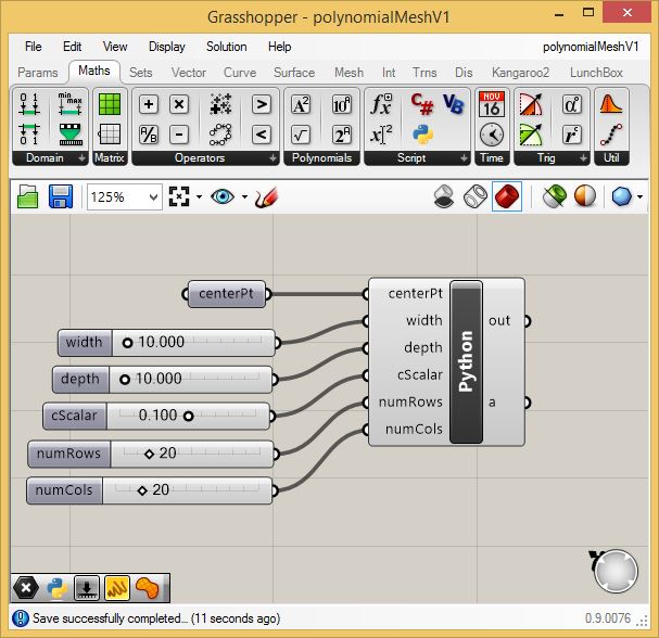
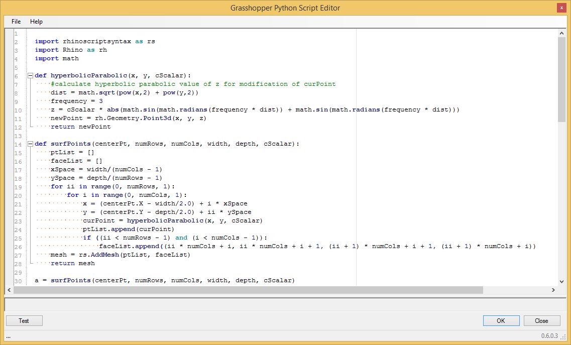
3. Create the following script within the Python component.
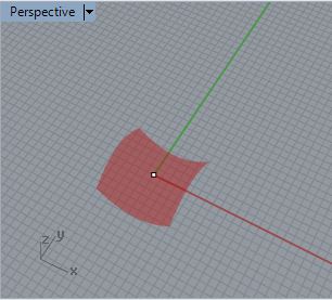
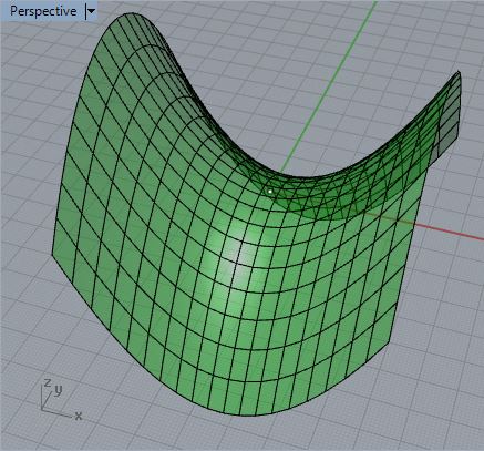
4. With parameters setup in part 3, baking the output of the component yields the following figure.
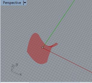
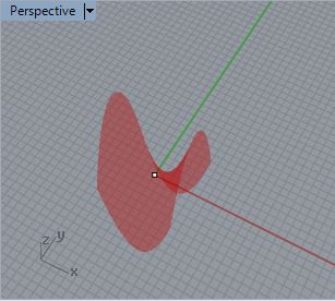
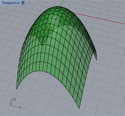
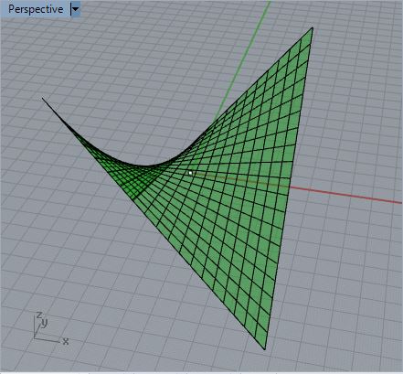
5. Varying the cScalar parameter setup in part 3 gives some of the following shapes (the view has been rotated to help see the resulting geometry).
 |
 |
 |
 |
| cScalar = 0.1 | cScalar = 0.25 | cScalar = 0.5 | cScalar =1 |
#Hyperbolic Parabolic Mesh |
 |
| #Eliptical Parabolic Mesh z = cScalar * (pow(x, 2) + pow(y, 2)) |
 |
| #Simple Saddle z = cScalar * (x * y) |
 |
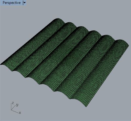
| #Sine Surface frequency = 2 z = cScalar * abs(math.sin(math.radians(x * frequency))) |
 |
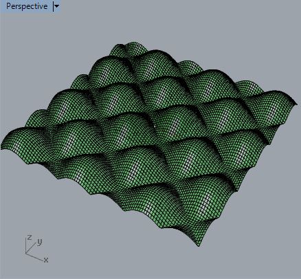
| #Sine Surface in X and Y frequency = 2 z = cScalar * abs(math.sin(math.radians(x * frequency)) + math.sin(math.radians(y * frequency))) |
 |
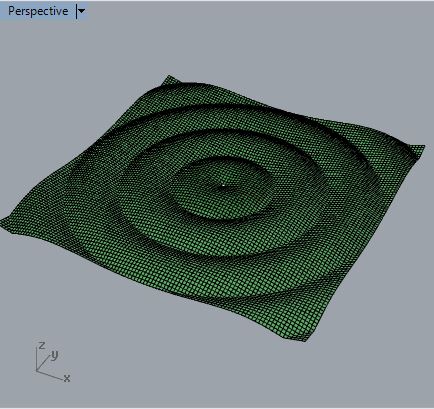
| #Concentric Sine Wave dist = math.sqrt(pow(x,2) + pow(y,2)) frequency = 3 z = cScalar * abs(math.sin(math.radians(frequency * dist)) + math.sin(math.radians(frequency * dist))) |
 |
Summary
Within this workshop we have developed a few basic scripts for representing three-dimensional surfaces . The principal building block of these surface elements has been a four sided polygon. We examined how such four side polygons could be arrayed together so as to create various kinds of polynomial based surfaces. The examples also demonstrate the power of encapsulating the basic parameters of a particular architectural composition within a few variables. In the case of polynomial related surfaces, we were able to succinctly describe the range of the surface (i.e., the variables width, depth), the scale of its curvature (i.e., the variable sScalar) and the resolution of its curvature (i.e., the variables numRows and NumCols).