COMPUTER
AIDED
ARCHITECTURAL DESIGN
Workshop 15 Notes,
Week of November 14 , 2017
VECTOR ARRAYS AND MAPPED OBJECTS TO 3D SURFACES
These workshop notes describe some commonly use techniques using vectors to translate objects. In
first two examples below, we set into place two similar 2D arrays that
produce the same result though related but distinct methods. In the
third example, we take on the more complex case of mapping of 3D object
(or collection of objects) to a doubly curved surface.
PART
1. 2D translation.
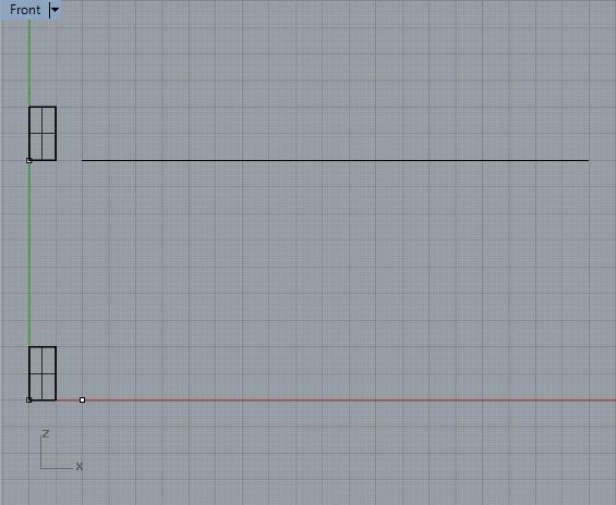
1. Within
this the front view place a 1' x 2' corner point to corner point
rectangular surface at the origin and one above it along the Y-Axis. In
addition, place points along the X-Axis at 0,0,0 and 0,2,0 and also one
at the lower left hand croner of the upper rectangle surface.
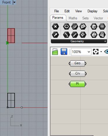
Now
open Grasshopper and put into place corresponding parameter
components. For the upper rectanglular suface at point create a Geo
component and pt as follows.
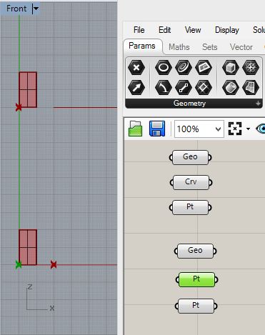
Similarly for the lower regtangular surface create a Geo component and two pt components:
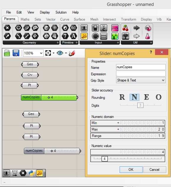
Next,
setup a number slider and rename it as "numCopies" for both
rectangular sufaces, with a range of 1 to 20 and a current value
of 4.
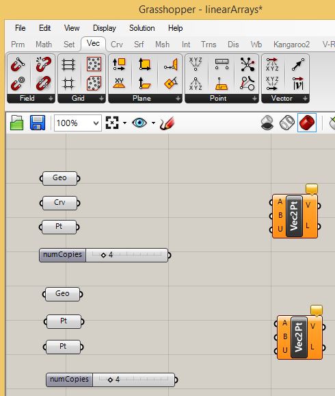
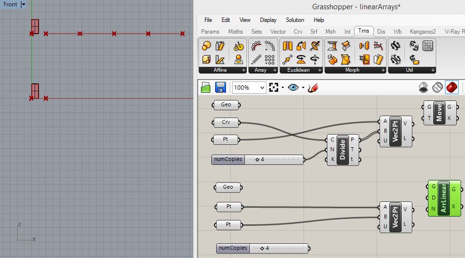
2.
Epand out the Grasshopper canvas window, and for the upper rectangular
surface, go to the vector tab and select the Vector 2 pt
component. Similarly create one fo the lower rectangular surface.
For
the upper rectanglar surface go the "Crv" tab, add a divide
curve component, and connect it to the "Crv" and
"numCopies" components. Furthermore, add and connect the "Vec2pt"
input port "A" to the original point at the lower left corner of
the rectangle and input port "B" to the output port "P" of the
"Divide" (divide curve) component.
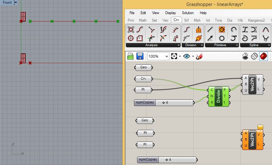
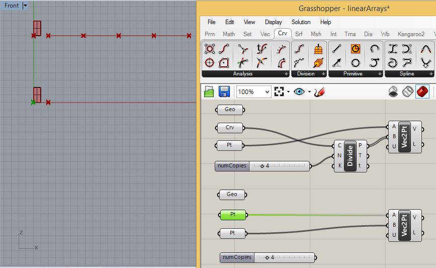
For the lower rectangle, connect the point parameters to the input ports "A" and "B" of the "Vec2Pt" component.
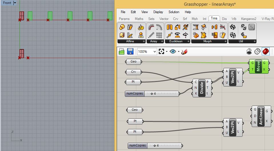
3.
Expand the visible Grasshopper canvas window area again, and now for
the upper rectangular surface, go the the "Trns" (transform) tab and
add a "Move" component. However, for the lower rectangular surface add
a "AriLinear" ( linear array) component.as follows:.
For
the upper rectangular surface connect the "Geo" parameter to the input
port "G" of the "Move" component and the output port "V" of the
"Vec2Pt" component to the input port "T" of the "Move" component.
Accordingly, the original rectangular surface copies and translates
along the horizontal line as follows:
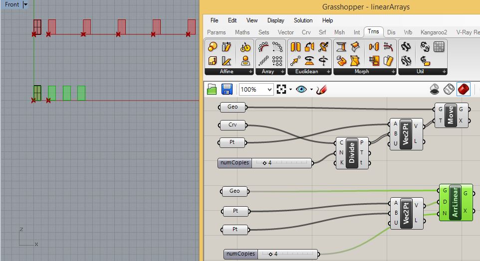
Similarly,
for the lower rectangular surface, connect the "Geo" component to
the input port "G" of the "AriLinear" component , the output port "V"
of the "Vec2Pt" component to the input port "D" of the
"AriLinear" components, and the output port of the "numCopies"
numerical slider to the input port "N" of the "AriLinear" component.
Accordingly, the original rectangular surface copies acccoring
the vector determined by the initial two points on the X-axis as
follows:
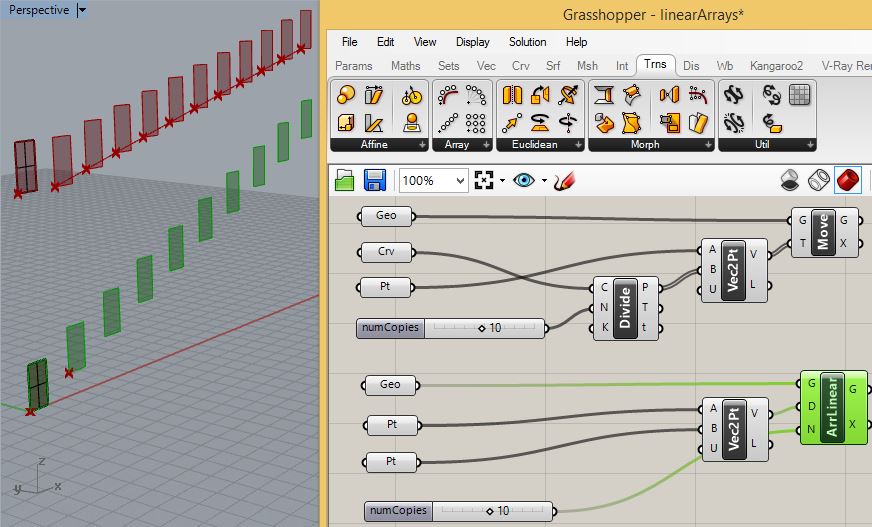
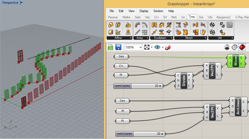
The
dynamics of tansforming the upper rectangular surface and of
translating the lower rangular surface are similar but the means are
distinct from one other. For example, for the upper rectangular
surface, you can rotate the line and increase the numbers of copies to
10, but for the lower rectangular surface, you can move the seond of
the two points to adust the vector direction and increase the
number of copies to 10.
The
same setup can also impact a translation of the rectangular surfaces
within to the X-Y plane. For example, for the upper rectangular
surface place a curve in the X-Y plane and use it to replace the one
attached to the "Crv" parameter. For the lower rectangular surface
surface, move the second point from its original location on the X axis
to new location in the postivie X-Y plane area. Increase the number of
copies for both to 20, and the result could be similar to the
image below:
PART
2: 3D Vector Mapping of Objects to Surfaces.
We
can apply a similar strategy to mapping an objecton the ground to
the UV coordinate system of a doubly curved surface and also taking
advantage of surface normals.
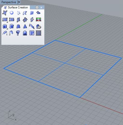
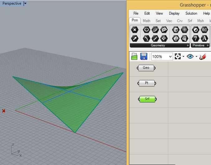
1. Create a 20 x 20 rectangular surface from the location 0, 0, 0 to the location 20, 20, 0 in the XY plane.
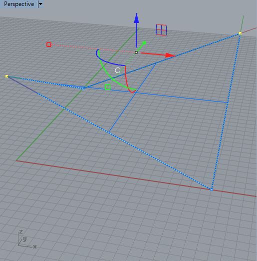
2. Turn on the control points and then select the ones on it's lower left and upper right corner in the X-Y plane. Wtih the Gumball tool move the control points above the ground plane to create a simple saddle shape.
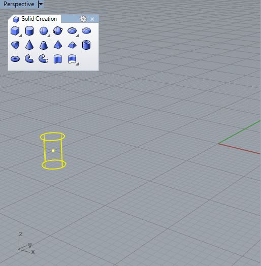
3
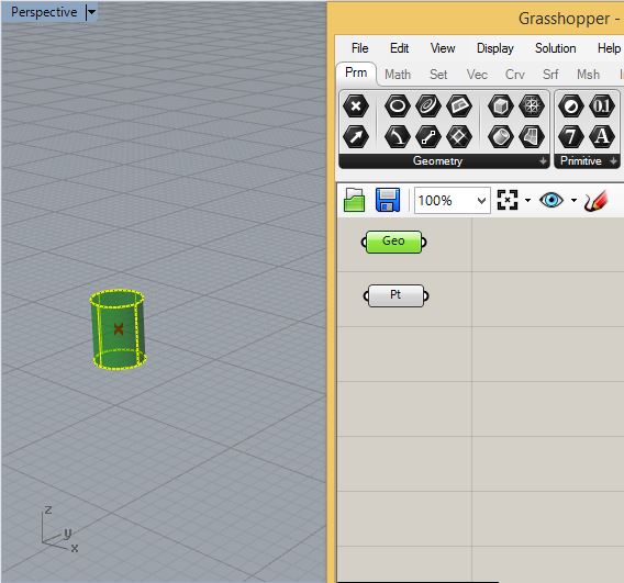
. Next place a point at at the location -2, -2, 0 and a solid cylinder
of radius 0.2 at the same location. Move the cynlinder downward so that
it is bisected by the ground plane.
Save the Rhino file, open Grasshopper and initiate a new Grasshopper file.
4.
Within the Grasshopper "Params" (parameter tab), add a "Geo" and
"Pt" component and connect them to the Cylinder and to the point in
Rhino respectively.
Similarly, add a surface component and connect it to the simple saddle shape.
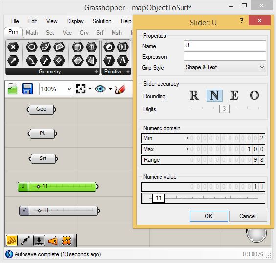
Add two integer sliders ranging in value from 2 to 100 and labelled "U" and "V" for the surface coordinate system.
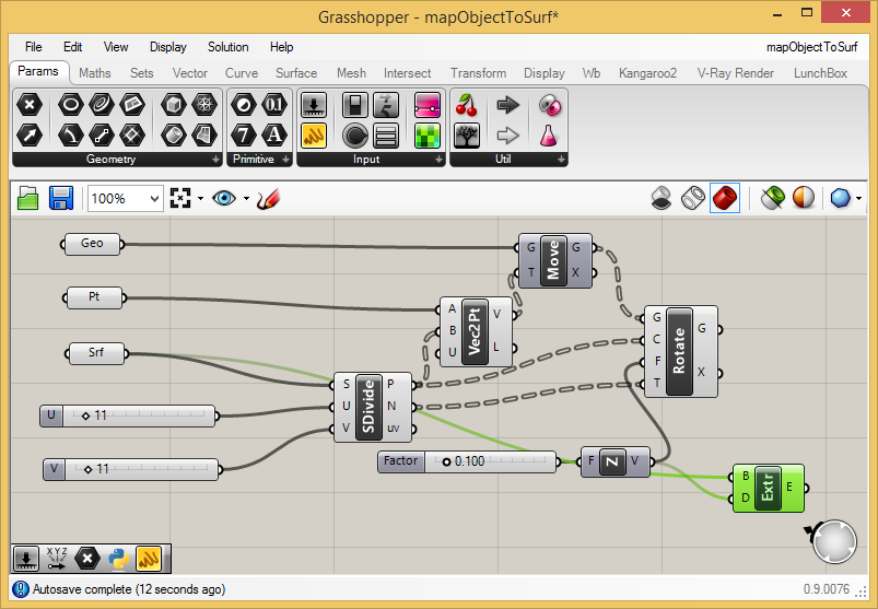
5.
In the next step we establish a set of vectors from the point at
the center of the cylinder on the ground to U V points along the
saddle surface. Begin by going to the "Surface" tab, and in the
area labelled "Uti" (utility) select a "Divide Surface" component (to
the upper left of the "Util" lable and place it in the canvas
window.
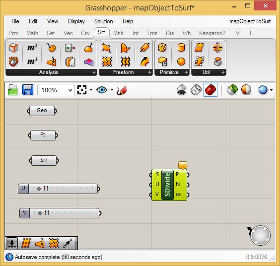
Connect
the "U" and "V" numerical sliders to the "U" and "V" input ports
of the "SDivide" (divide surface) component, and also connect the
"Srf" component to the "S" input port of the "SDivide" component, and
see the points generated along the saddle shape. The grid consists 11
spaces along each side of the surface as defined by 12 points (there's
always one more point than the number of spaces).

Similar
to Part 1 and the previous linear array example go to the "Vec"
(vector) tab and place a point to point "Vec2Pt" vector component in
the canvas window.
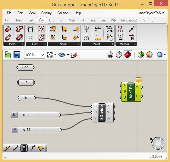
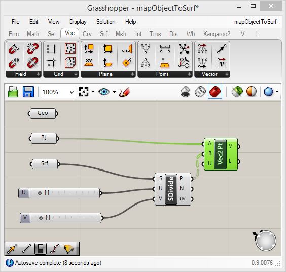
Connect
the original "Pt" component that was connected the point located at the
center of the cylinder to the input port "A" on the "Vec2Pt" component,
and connect the output port "P" of the "SDivide" component to the input
port "B" on the "Vec2Pt" component.. Note that the double line
connecting port "P" to port "B" indicates a list of points coming off
the saddle shape rather than a single point.
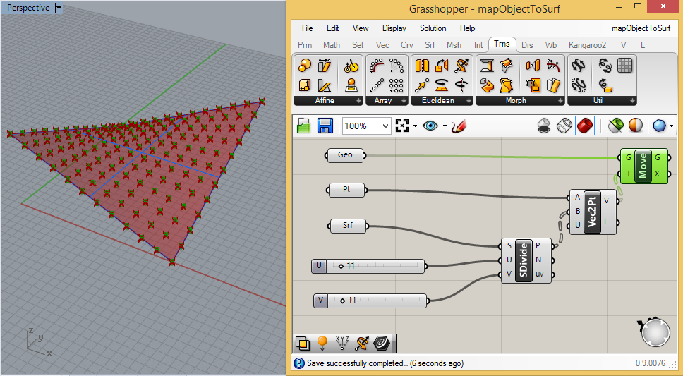
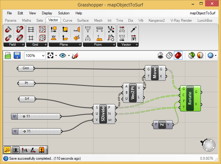
Now
go to the "Trns" (transform) tab, and from above the "Euclidean" area
add a "Move" component (the orange arrow symbol between two white
dots). Attach the "Geo" component to the input for "G" of the "Move"
component, and attach the output port "V" from the "Vec2Pt" component
to the input port "T" of the "Vec2Pt" component. When completed, the
cylinders will map to the U V points on the saddle shape. They will
also bisect the saddle shape similarly to how the original cylinder is
bisected by the point on the ground and at its center.
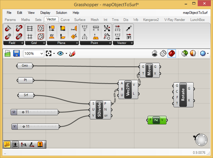
Upon
closer examination, however, the cylinders are perpendiclar to the
ground plane and not to the surface locations where they are mapped. In
order to address this we can rotate them from their current orientation
to the orientations of the surface normals. First, staying witin the
"Trns" tabl, select the down arrow in the "Euclidean" and then the
"Rotate" icon that has one vector rotating towards another one with
input ports G, C, F, and T. Next, returning to the "Vec" tab and the
icons that can be viewed by selecting the down area labelled "Vector"
on the right hand side, add a "unitZ" vector to the canvas window
as highlighed in green below.
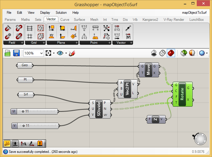
To
activate the rotation of the cylinders, connect the output port "G"
from the "Move" component to the input port "G" of the "Rotate"
component, connect the output port "P" from the "Subdivide" component"
to the input port "C" (Centers of rotation) of the "Rotate" component, connect the output port "N" (surface Normals) to the input port "T" (the vector to rotate To)
of the "Rotate" component, and connect the output port "V" of the
"UnitZ" component to the input port "F" (the the vector to rotate From) of the the "Rotate Component".
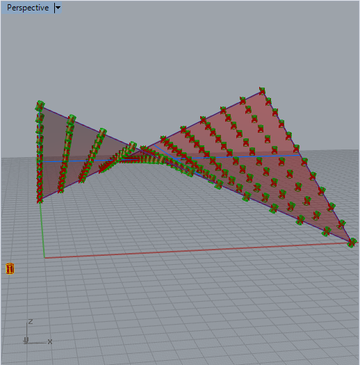
To
separate out the rotated cylinders from the original ones, turn off the
"preview" option on the "Move" component (right-mouse-click on the word
"Move" and then left-mouse-click the "Preview" option off).
Note that the cylinders are now all colinear with the surface normals.
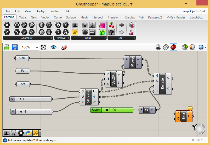
6.
In the next step we thicken the surface to setup for subracting the
cylinders from it. Returning to the "Surface" tab and under the
"Freeform" area select the "Extrude" component and place it to the
right of the "UnitZ" component. In addition, return to the
"Params" tab and add a number slider to the left of the "UnitZ"
component. The slider should range in value from 0.0 to 1.0
(its default seeing). Connect the slider output to the input "F"
(factor) component of the
"UnitZ" component. The factor will serve to mulitple the vector. Since
the vector is originally a "unit" vector (a vector of length 1.0), the
factor will change
it's length to the value of the slider (0.1 in the case below).
To
comlete this step, connect the output port "V" of the "UnitZ" component
to the input port "D" of the "Extr" (extrude) component and
connect the saddle surface "Srf" component to the input port "B"
(boundary representation, i.e., the surface) of the "Extr" component.
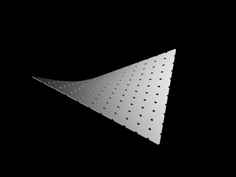
The
Rhino perspective view window will now show that the saddle surface has
thickened into a solid from which it will be possible to subtract the
cylinders. Note that if you wish to have the cylinders push through the
lower and upper sides of the saddle surface, you may need to adjust the
height of the original cylinder. The changes will automatically
propagate to the ones mapped to the saddle surface.

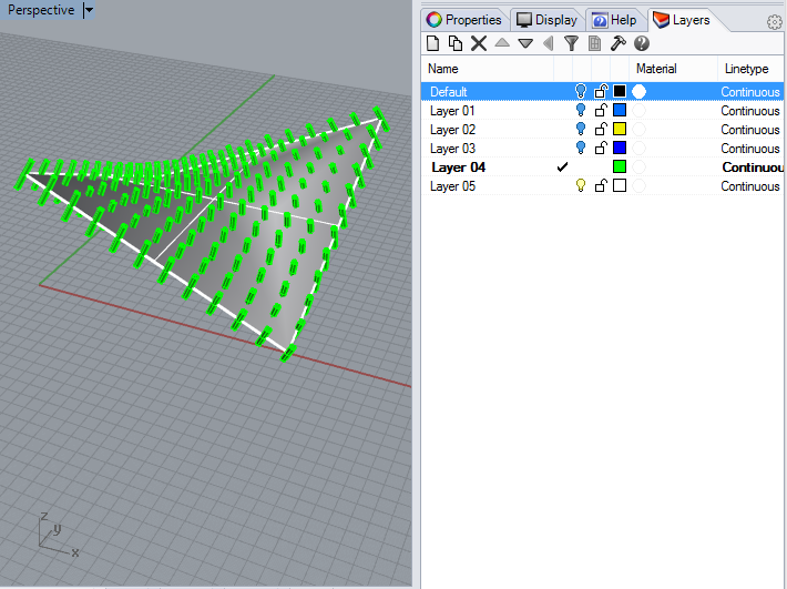
7.
First, if necessary, extend the vertical heightt of the original
cylinder with the Gumball tool to ensure that its translated instances
push through both its upper and lower sides of the saddle solid
shape. Next, to complete the solid subtraction, bake the
thickened saddle surface to one layer inside Rhino (e.g., layer 4), and
bake the normalized cylinders to a separate layer (e.g., layer 5). That
is, proceed by right-mouse-clicking on the "Extr" component over the
letter "G" and using the left-mouse-button to select the "bake"
option. Similarly, select the letter "E" on the "Rotate"
component, and bake the output (the cylinders) to a separate
layer. Turning off the layers for the original cylinder and for
the original saddle surface we get the result below in the perspective
view window.
8.
Continue in Rhino with the Solid Tools and the Boolean Difference
operator (second icon first row in the popup menu shown below). When
prompted at the Rhino command prompt for the surfaces to "subject from"
select the thickened saddle shape.
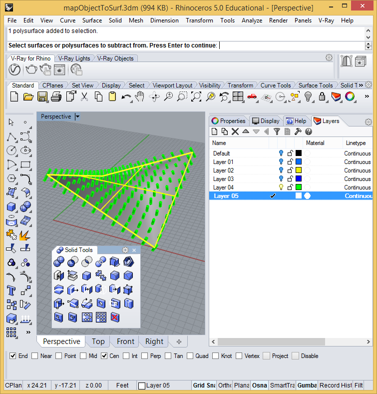
After
pressing the enter key and when prompted at the Rhino command
prompt for the surfaces to "subtract with" right-click on
the cylinders layer (e.g.. layer 04) and choose the option to "select
objects on layer". Note also that it would be best to also use
the "DeleteInput=Yes" option at the command prompt so that all
that remains after the difference operation is completed is the saddle
shape with the subtracted holes.