COMPUTER AIDED ARCHITECTURAL DESIGN
Workshop 2 Notes,
Week of September 3, 2018
Graphics Primitives Continued, Symmetry Operations, Modify and Select Tools
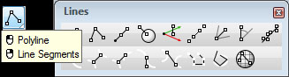
1. PRIMITIVES REVIEW
Primitives consist of basic elements such as lines, circles, arcs, boxes, etc.
Primitive tools typically have options associated with them to
control the method of primitive creation (ie. a circle by edge, center,
or diameter, copy, etc.). Remember to use the appropriate icon under
the subtools to control
the ways in which these elements are defined. Depending on which method
of definition you are using, the command prompt has default options
(such as a circle being 1'-0" in diameter), but can be overriden by
keying in a specific dimension or control.
![]()
2. TOOL BOX ORGANIZATION
Within the tool bar, additional sub tools can be accessed by holding down the left mouse button on any tool icon with a triangle in the lower left hand corner. For example, by selecting the line icon, a sub-tool palette below can be pulled out and displayed as its own tool bar as well.
Defining your own toolbar: You can create your own toolbar by going to Tools / Toolbar Layout. You should first go to File / SaveAs to save your own toolbar collection so as to not edit the existing default one. After you've saved the toolbar to your folder, go to Toolbar / New and define the name of your custom toolbar. This will create a new floating window in which you can copy any icon over to this location. To do so, use the CTRL key on your keyboard and drag a duplicate icon you want here.
Go to Tools / Lock Toolbar if you wish to lock the toolbar locations.
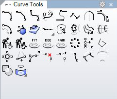
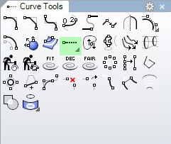
3. CURVES
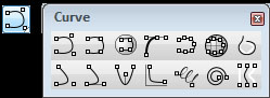
Control Point Curve (the first icon in the Curves subtool palette): This is a line based, simple curve that is very quick, but does not provide a lot of control or exact geometrical specification. You can control the degree of the curve in the command prompt.
Interpolate Curve (the second icon in the Curves subtool palette): The curve is drawn by points which are directly in the path of the curve. This will create a closer fitting curve to specific points. However, this results in a curve that is typically less smooth than the Control Points curve.
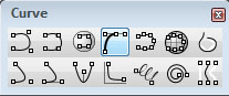
Handle Curves (icon highlighted above). With Handle Curves, the curve is defined by tangential lines. The length pf the tangent lines effects their impact on the curve.
OBSERVATION: When constructing a curve, don’t
just trace a drawing. Work to figure out the geometric elements most
descriptive of the design. This may help you to more completely
understand the geometrical order of the design, and later optimize on
finding a more advanced and appropriate technology to use (i.e. spiral
tool
for the Guggenheim ![]() ). That is, test varied type curves to substantively work
through the goeometrical composition.
). That is, test varied type curves to substantively work
through the goeometrical composition.
NOTE: any of these tools can be used through typing in the command prompt.
4. LAYERS
![]()
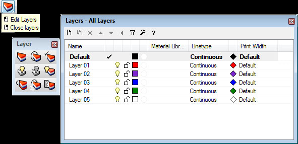
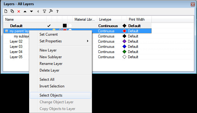
Click the colorful pie wedge icon on the top toolbar to bring up the layers window. You can dock it anywhere on the screen.
Double click on a layer to make any layer active (signified by the check mark), and turning the lightbulb icon on/off will control visibility of that layer. Using layers allows parts of the model to be turned off or on and will be useful for assigning attributes, such as assigning colors of lines or linetypes. You can select multiple layers by using the SHIFT (adjacent layers) and CTRL (individual layers) keys.
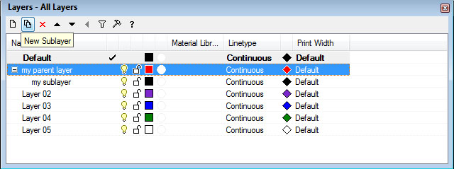
To create a new layer, select the new level icon in upper-left corner, and enter into the text box for the new layer any aribitrary name ( e.g., "my parent layer").
To create a sublayer, select the parent layer, and click on the New Sublayer icon. You can use the up and down icons to adjust the layer hierarchy.
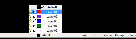
Shortcut: Quickly make a layer active by clicking on the layer name in the status bar located at the bottom of the Rhino window.
By best practice, each level in Rhino should be given
an independent color so as to be able to more easily understand the
organization of drawing. To begin, create a new level for each
different type element of your drawing (e.g, walls, roof, etc..). Work
this way from the outset in order to keep in place an ongoing
conceptual framework of the organization of your model. It may be that
you will adjust this framework as your model develops or as new ways of
parsing your project
occur to you.
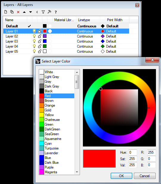
To choose the color per layer, simply click on the square next to the
lock key. For example, pick color (i.e., red)
for the given level (i.e., "Layer 01") as shown in the dialog box
below:
Furthermore, you can set the properties for the
material assigned to that layer by selecting the circle icon next to
the square above. You can also set the linetype and print color as well
as print width here.
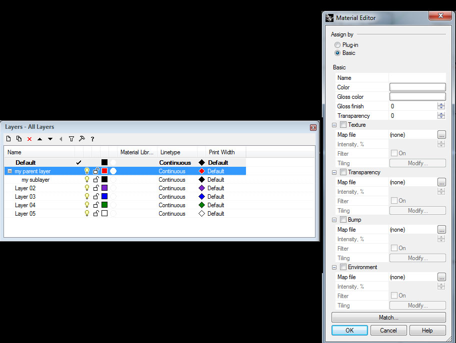
To select all objects on any layer, right click on the layer name and select "select objects".
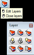
Other ways of using layers can be found in the subset tool palette for Layers. First select the objects to modify, then use the icons to do the following:
Edit Layers : as described previously
Change/Modify Object Layer
Set Current Layer
One Layer On/Off
Duplicate Layer
Copy Objects to Layer
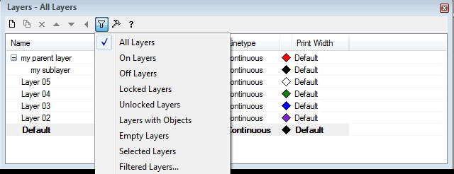
5. Using Filters to show the layers that match the following properties.
6. SELECTING OBJECTS:
Edit select by attributes: Open up the subpalette for the following tool icon:
Most are self explanatory (Select all, none, inverse, etc.), but here are some specific tools that are helpful to know:
Select Duplicate
Select by Color
Select All Block Instances
Select Curves to open a sub palette to see options for selecting Short, Open, Closed curves, or polylines.
Select Chain: Selects curves or surface edges that touch end to end.
Drawing a box to select objects in your model.
NOTE: Use SHIFT to add/remove objects from your selection. You can pre-select before using other tools to alter more than one element at a time.
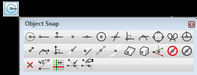
7. OBJECT SNAP TOOLS
Recall from the last
workshop how the OSnap toggle control on the status bar at the bottom
of the screen is a quick way to use snaps. An alternate and more
detailed way to do this is to select the icon in the standard toolbar
(towards the top of your screen) to see other methods of object
snapping.
Note: Persistent object snaps (right clicking on these snap icons) maintains an object snap through choosing several points without having to reclick the snap tool.
6. SYMMETRY TOOLS (Move, Rotate, Mirror, Scale, etc.)
Copy element. Method: type in # of copies in dialog box if more than one copy is desired at the same distance from one another.
Move element tool is vector based and can be translated from a point not within the object being modified. Click on or outside element once it’s selected and move in desired direction, typing in distance in Accudraw if you like. The Move element tool can be used with copies and with repititions by selecting the appropriate options in the dialog box.
Scale tool can be used with numeric input or the three point method. This tool can also be used with repetitions. Open the tool subset to have options for scaling 3D, 2D, 1D (stretching), and non-uniform.
Rotate tool can also be used with copies and repitition. To rotate an object to a specific angle, type the angle number in the dialog box after selecting the object to rotate.
Mirror tool can be used to make an exact mirrored copy of a desired object along a selected axis.
Rectangular Array (open up tool subset to see options for arraying along a curve or surface)
Polar Array
Make sure to pay attention to the command prompt for the specific usage steps of each tool.
NOTE: any of these tools can be used through typing in the command prompt.
7. SOME MORE CURVES
Helix, Spiral, and Average Curves (last 3 icons):
Average Curves (averages two curves)
8. MODIFY TOOLS
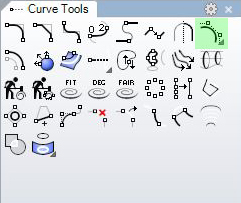
Under the main2 toolbar (left side of screen), pull out the curve tools icon:
Extend line extends a line.
Circular Fillet through a defined radius
Construct Chamfer
Offset element by distance
Close Open Curve
Curve Boolean (combine regions)
The pull-down menu from the icon in upper right-hand corner leads to following sub-menu to edit points on curvess: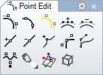
Insert/Delete control point (from point edit sub-palette)
Additional Modification Tools in the Main1 and Main2 toolbars on left hand side of screen:

Join - connects objects together to form a single element (for lines, curves, surfaces, polysurfaces, solids)
Explode - breaks objects down into components
Trim - deletes slected portions of an object where they are intersected with another object
Split - divides NURBS into parts by using elements to cut
NOTE: any of these tools can be used through typing in the command prompt.
TIP: Another way of quickly modifying control points on objects is by using the F10 key on the keyboard to display these points, and F11 to turn the points visibility off.
9. BLOCKS vs. Group/Ungroup
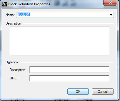
1) Blocks creates a single unit from selected objects. The object has an assigned name and is stored in the block library. You can update all instances of a block by modifying a block definition.
Defining a block: Type "block" in the command prompt, or open up the toolbar Block. Select elements to be blocked together and define a base point as per the command prompt. Assign a name, description as desired. Use link to link to external files. To refine a block, just use this same process but re-use the same block name.
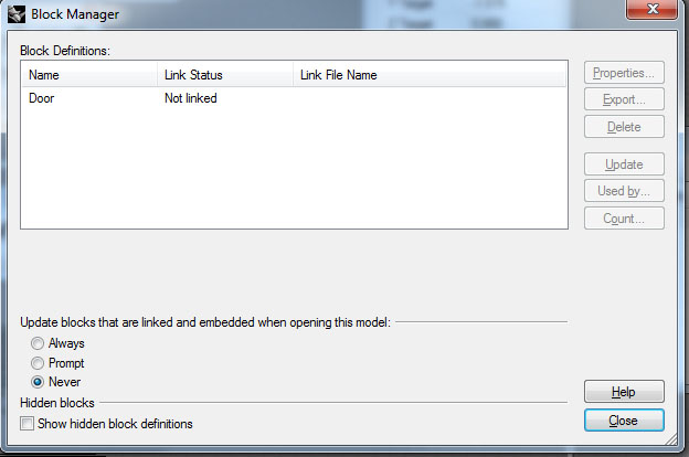
Use the "block manager" to see all the blocks defined in your file. Here you use the counter to see how many of each block object are in your file.
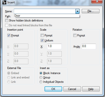
Key in "insert" in the command prompt to insert a defined block into your model.
2) You can use the Group/Ungroup icons in the Main1 and Main2 toolbars on the left side of your screen to create a single unit from selected objects.
10. Catenary curve.
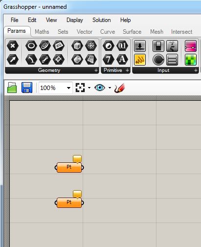
Create two points at arbitrary locations in the plan view in Rhino.
Similar to the steps outlined at the of workshop 1, at the command type in "Grasshopper" to load the plugin, and from the Parameters (Prm) tab, place two point symbols in the Canvass window.
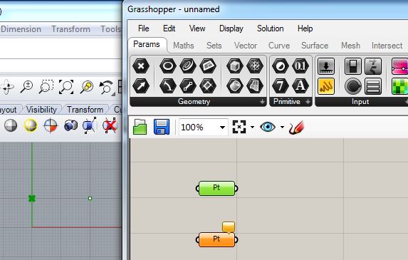
Right-click on the first "Pt" symbol and choose "set one point" and using the mouse select the first point in Rhino (note that you can either select the point directly with the left mouse button, or drag a "rubber banding" window around it inside Rhino.):
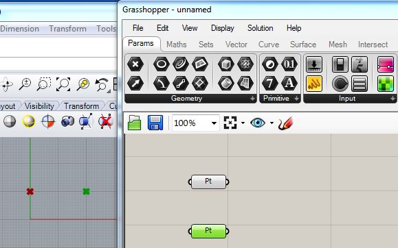
Repeat this so as to connect the second "Pt" symbol with the second of the two points in Rhino.
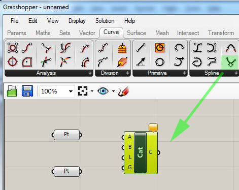
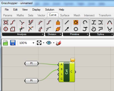
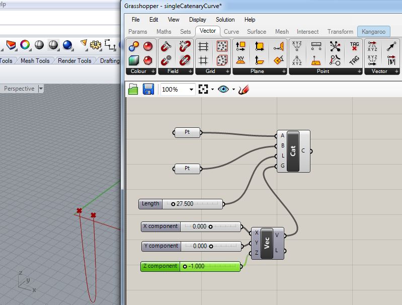
Within "Grasshopper" go to the "Curve" tab, and from the "Spline" area select the "catenary" curve symbol and drag it into the "canvass" window:
Connect the output port of the first "Pt" to the input port "A" of the "cat" symbol, and connect the output port of the second "Pt" to the input port "B" of the "cat" symbol:
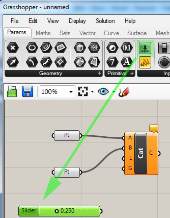
Return to the "Params" tab and drag a numerical input slider into the canvas area:
Double-click with the left mouse button directly on the text " slider", set its range to be 5 to 150, set its value to 27.5, and connect its output port to input port "L" of the "cat" symbol.
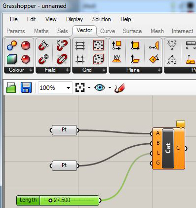
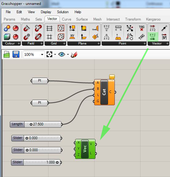
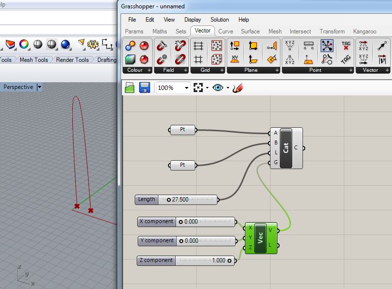
Add three more sliders without modifying their default value ranges. Next, go to the "Vector" tab, and add a construct vector "symbol" to the canvass.
Change the values of the three new sliders to 0.0, 0.0, and 1.0, and connect them to the "X", "Y" and "Z" input ports of the Vec symbol. Next, connect the "V" output port of the "Vec" symbol to the "G" input port of the "Cat" symbol. Note that a catenary curve is now generated from the two points draping in the negative "Z" direction:
Change the range of each X component, Y component, and Z component sliders to go from -1 to 1. Change their current values to 0.0, 0.0 , and -1.0 respective and note that the catenary curve hands as if pulled in the negative "Z' axis by gravity.
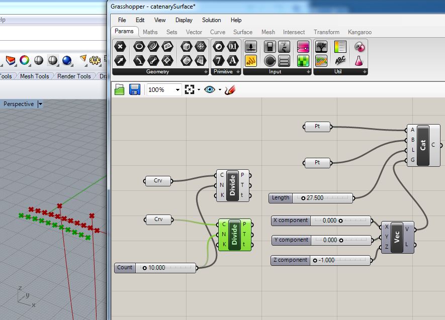
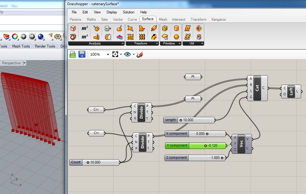
11. Catenary curve series.
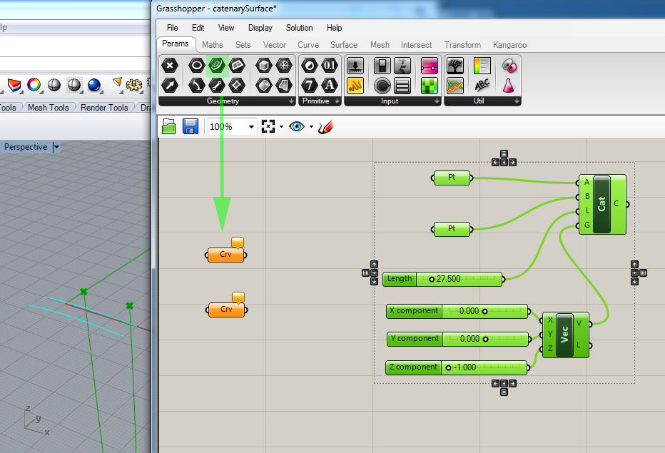
In this example, we add draw two simple parallel curves (shown in blue-cyan in the perspective window below) in the plan of the same Rhino model used to draw the single catenary curve. We then go to "Params" tab, and drag a "curve" symbol into the "canvass" window. Note that in this illustration we also use the mouse to drag a rectangle around the other symbols in the "canvass" window, and then move them to the right to make way for the two new "curve" symbols.
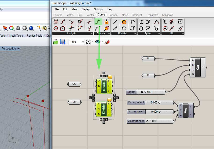
Connect the two new curves to the "Crv" symbols in the "canvass" window. Go to the "Vector" tab, and add two "divide curve" symbols:
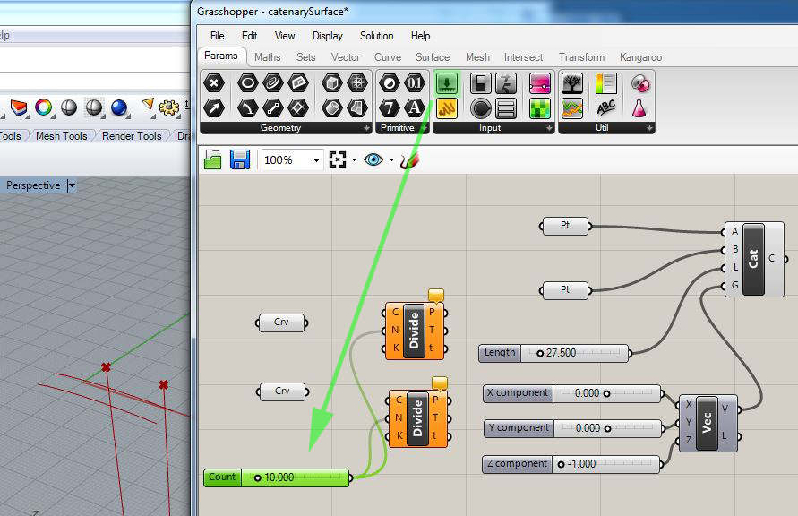
Return to the "Params" tab" and add a new numerical input slider with a range in values of 2 to 100, and set its output port to the "N" input ports of both of the "Divide" symbols.
Now, connect the output ports of each of the two "crv" symbols to the corresponding input ports "C" of the "Divide" symbols, and series of points is create along each of the two new curves added to the Rhino model.
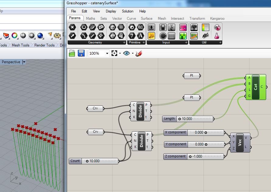
Connect the output ports "P" of the two "Divide" symbols to the corresponding input ports "A" and "B" of the "Cat" symbol. This connection now supplants the connections from the original two points in step 10 above, and a series of Catenary curves is now created. Note too that in this example the "length" slider is reduced from 27.5 to 10.0.
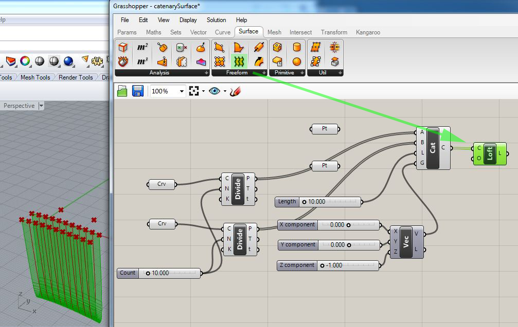
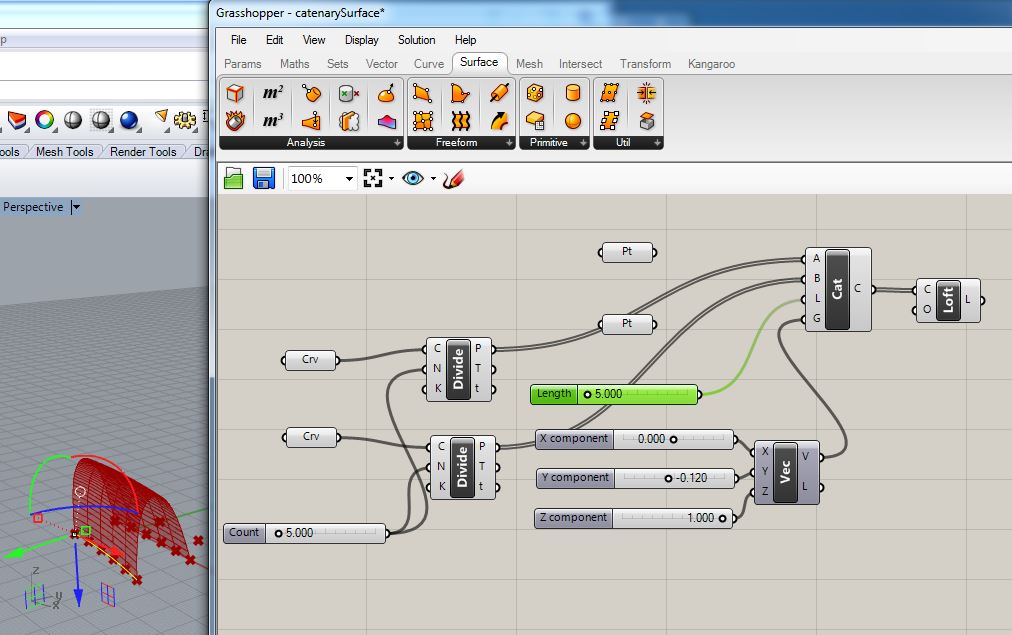
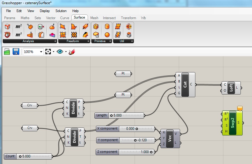
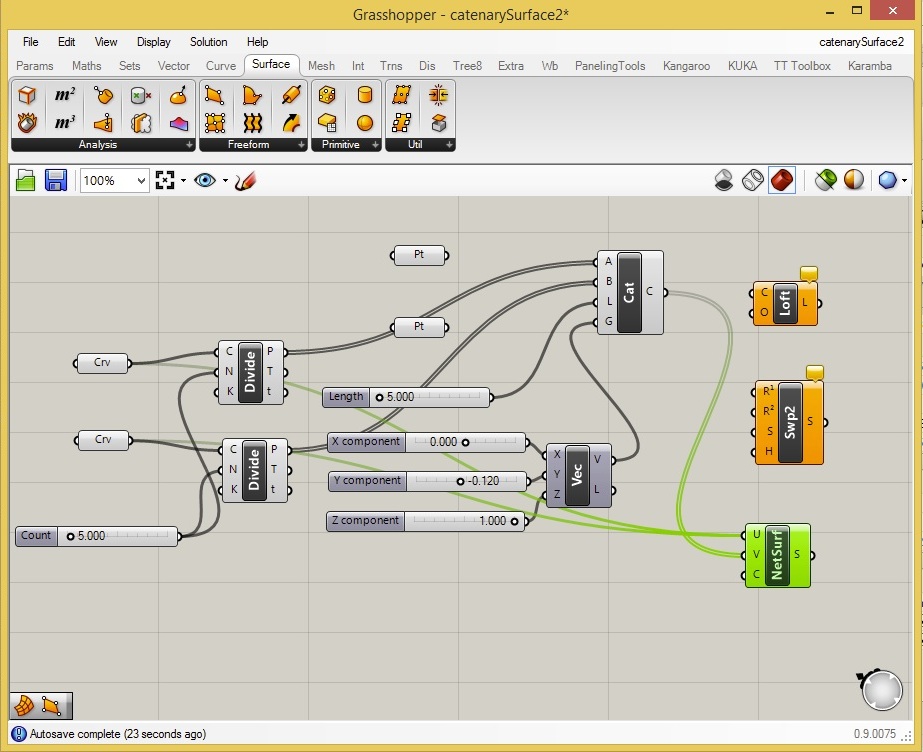
12. Catenary curves to lofted surface.
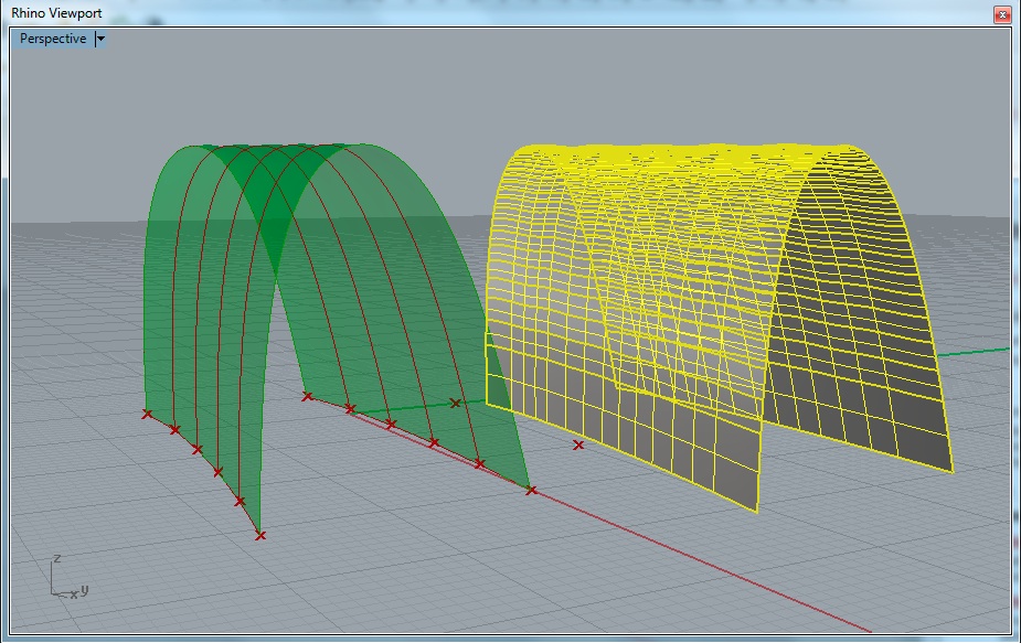
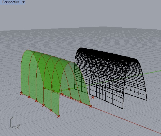
Note that two methods of generating the surface are shown below. The first method uses a "loft" surface. Note that the curves must be relatively simple for this technique to work.There's a risk that the surface may fold in on itself. If that occurs with the "loft" surface, then try using simpler curves or lessening the "Length" input parameter to the "Cat" symbol. The second method, described further below, uses a "bi-rail" surface which is more likely to result in a coherent surface that isn't folding in on itself. Both methods are shown below. The second method results in the Grasshopper file catenarySurface.gh based upon the Rhino file makeCatenarySurfaces.3dm (right-click and do a "save as" on these links to download the files). A third option, not shown, involves creating a procedure in the Visual Basic" component to Grasshopper that parses the series of catenary curves into a series of adjacent pairs and then generates a series of surfaces rather than a single whole surface.
12.1 Loft surface: continuing with the the last example of step 11, go to the "Surface" tab inside of Grasshopper, and add a "loft surface" symbol to the right of the "Cat" symbol. Connect the output port "C" of the "Cat" symbols to the corresponding input port "C" of the "Loft" symbol. This connection generates a suspended catenary surface from the two curves.
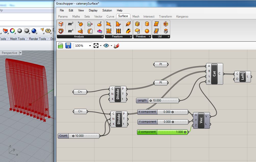
Adjust the value of the "Z component" slider to 1 to have the catenary curve move in the positive "Z" direction.
Adjust the value of the "Y component" slider to -0.12 to cause the catenary curve to lean slighty in the negative "Y" direction.
Explore variations in the other numerical sliders, including the "count" slider to see how the surface is modified. Similary, move or rotate slightly either of the two curves in Rhino and see how the changes in the surface are automatically generated. For example, move the curves in the ground plane further apart, rotate one slighlty, change the number of catenary curves to 5, and the length to 10.
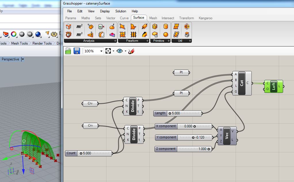
To import the surface more completely inside Rhino, right-clock on the "Loft" symbol highlighted in green below and from the popup dialog box that follows (not shown below) select the item "Bake".
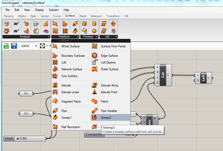
12.2 Method 2: BiRail by 2 Rails
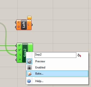
In Grasshopper, to the "Surface" tab, and pulling down the "Freeform" sub-tab, left-click on the "Sweep2" icon and drag it into the canvas window:
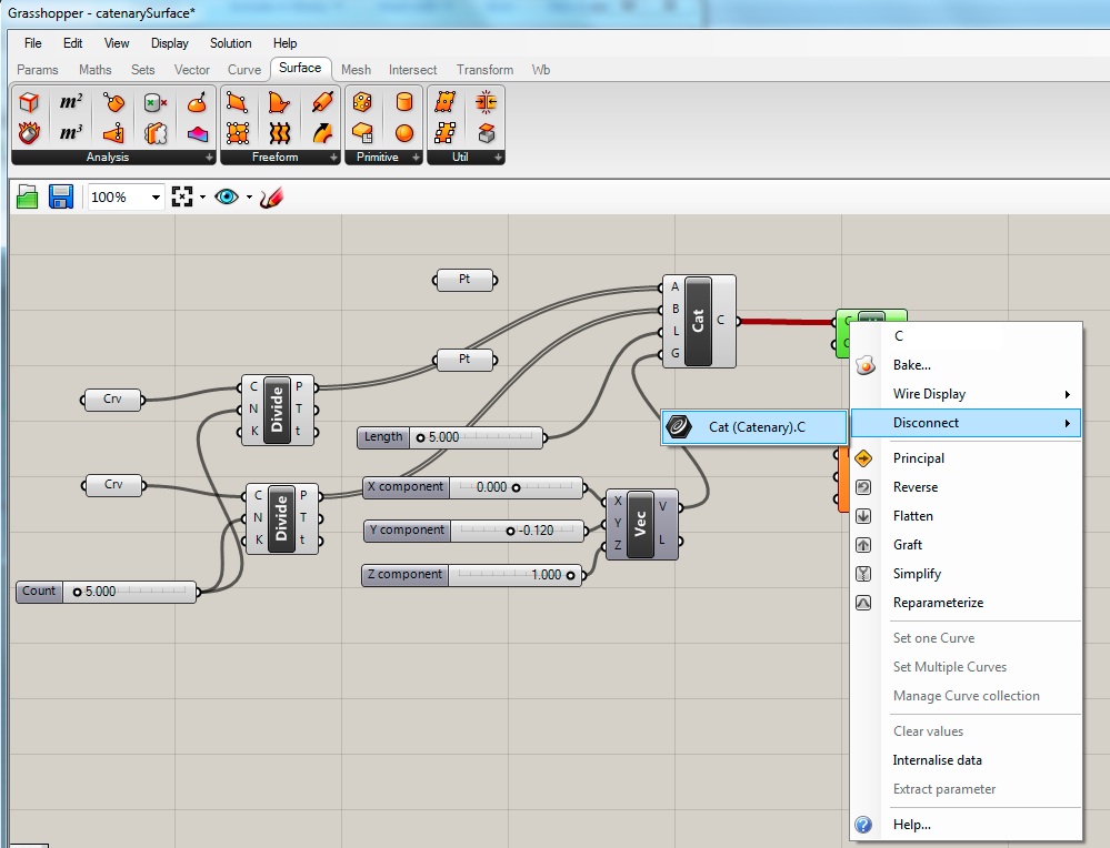
The Birail surface component, shown in green below, has inputs labelled "R1" and "R2" for the two "rail" curves, and "S" for the catenary curve sections:
First, within the "canvas" window, right-click on the "loft" component, and select the "disconnect input" option to remove the catenary curves as input.
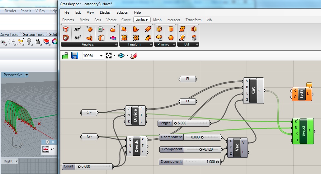
Next, connect the two "crv" components to "R1 and "R2" and also connect the output port "C" of the "Cat" component to the input port "S" of the "Swp2" component.
Finally, right-mouse click on the "Swep2" component, and left-mouse click on "Bake" to fully import the surface into Rhino. Once imported, the "baked" surface can be moved and treated like any other polygon surface.
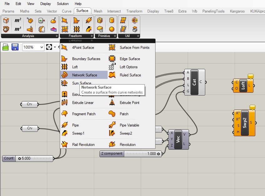
12.3 Method 3: Network surface.
Depending upon the character of the initial curves on the ground, the second method may sometimes also fail. A network surface is yet a third surface type within Grasshopper that tends to be more robust in these additional sitautions. The surface is compiled from two sets of curves moving in relatively perpendicular directions along the surface, the U and the V directions. Similar to the other two methods, the first step is to go to the "Surface" tab within Grasshopper, and pulling down the "Freeform" sub-tab and left-click on the "Network Surface" icon and drag it into the canvas window:
The "Network Surface" component, shown in green below, has inputs labelled "U" and "V" for the two sets of curves. Connect the one of the original "crv" output ports to the "U" input port of the Network Surface. Next, holding down the "shift" key, connect the other one of the "crv" output ports to the "U" input port of the Network Surface. By using the "shift" key, it's possible to add on the second "crv" to the "U" input port without disconnecting the first one. Next, drag the output port "C" of the catenary curves to the input port "V" of the "Network Surface" component.
The network surface will now be generated within the Rhino drawing window. Finally, right-mouse click on the "S" output port of the "Network Surface" component, and left-mouse click on "Bake" to fully import the surface into Rhino. Similar to the previous two examples, once imported, the "baked" surface can be moved and treated like any other polygon surface.
This grasshopper file catenarySurface2.gh contains surface components corresponding to the three different methods outlined here. The surface components for the first two surface types have been disconnected from the curve input data, and the component for the third surface type has been connected to this data.
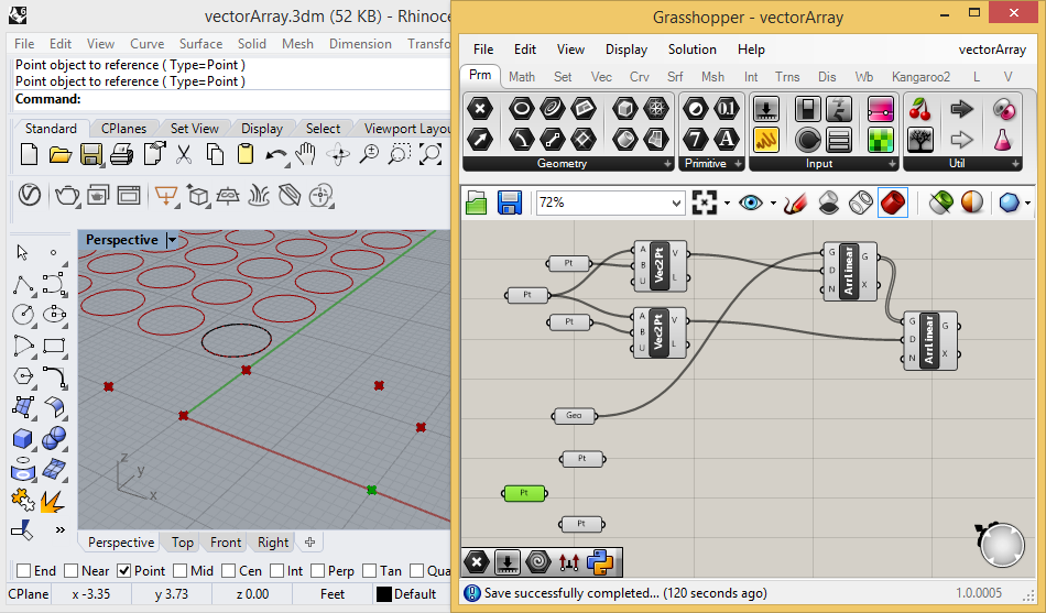
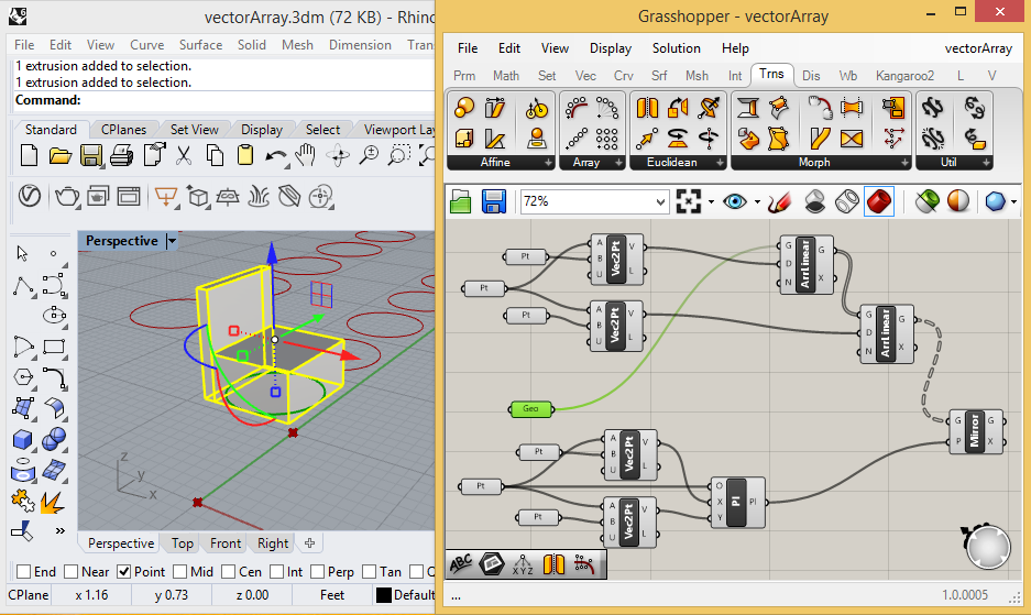
13. Vectors and Arrays
Steps 13, 14 and 15 produce a grasshopper file that mirrors seating. It would be best to reconstruct the steps in the order illustrated here. However the completed Rhino file vectorArray.3dm and associated grasshopper grasshopper file vectorArray.gh are included here for edification.
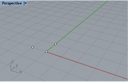
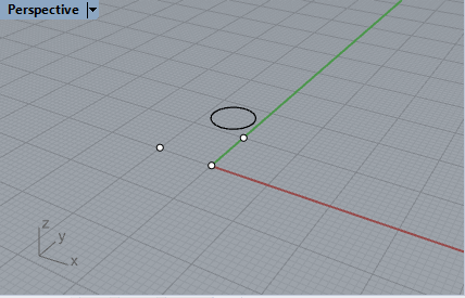
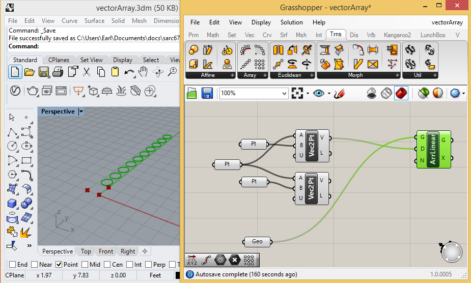
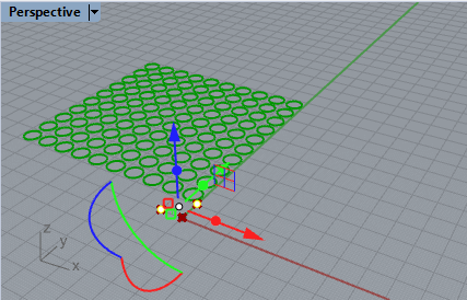
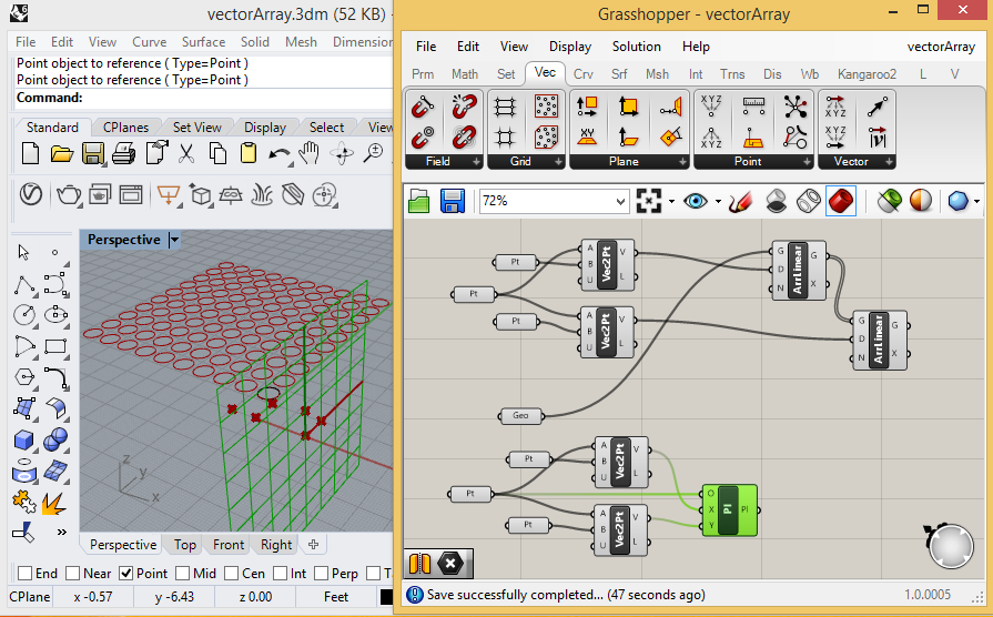
Within this example we examine the use of vectors to generate an array of objects, and also to facilitate a mirror of that array. Begin in Rhino with drawing three points at the locations (1) 0,0,0, (2) -1, 0, 0 and (3) 0, 1, 0 in the ground plane of the world coordinate system as shown in the figure below.
Next, place a circle centered on the location -0.5, 1.5, 0 of radius slightly less than 0.5 as depicted below.
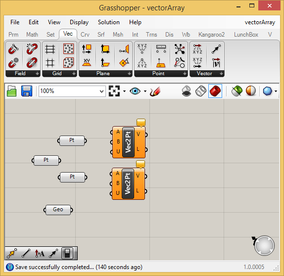
Now type "Grasshopper" at the command prompt to open up the Grasshopper application window. Forom the Grasshopper "Param" tab, place thee "point" components and one "geometry" component in the canvass window. Note that the "geometry" component is located within the sub-menu that appears below the word "Geometry" on the left-hand side of the Grasshopper dialog window.
Associate the first point "Pt" component above with the point 0,1, 0 in Rhino along the y-axis, the second point "Pt" component above with the point 0,0, 0 in Rhino on the x-axis, and the third component point "Pt" above with the point -1,0,0, in Rhino along the negative x-axis by using the same method as illustrated in step 10 . catenary curve example above. SImilarly, connect the "Geo" with the circle created in Rhino.
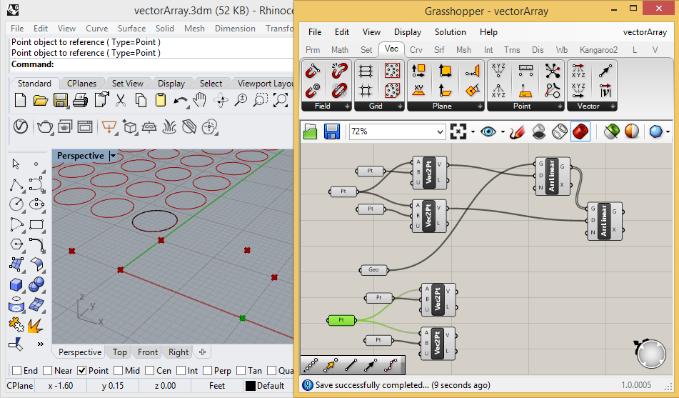
SImilarly continuing within Grasshopper, go the vector tab, and on the right-hand side, upper right-hand corner, select the vector created by two points component (a black diagonal arrow symbol with two white dots), and place one adjacent to the first "Pt" component and a second adjacent to the second "Pt" component in the Grasshopper canvas window. At this point also begin to safeguard your work by saving the Rhino file as "vectorArray.3dm" and by saving the Grasshopper file as "vectorArray.gh".
The "Pt" component in the center should be connected to input port "B" of both "Vec2Pt" components forming the start of each vector, and the other "Pt" components should be connected to the input port "A" of each corresponding "Vec2Pt" conponent to create a unit 1 length vector along the positive Y and one along the negative X axis respectively.
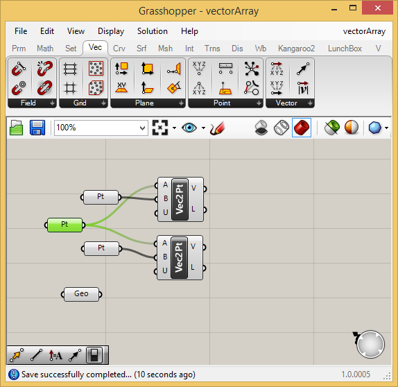
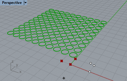
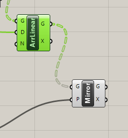
Go to the "Trans" tab (also abbreviated as "T" on a smaller Grasshopper window) and select the "Linear Array" component just to the upper right of the word "Array" and place it in the canvas window just to the right of the first "Vec2Pt" component.
Connect the "V" output port for the first "Vec2Pt" component into the "D" (direction) input port of the "AriLinear" component, and connect the "Geo"component into the "G" (geometry) input por the "AriLinear" component. For the time being the "N" (number) input port into the "AirLinear" component will be unconnected so that the default value of "10" array elements will be in effect.
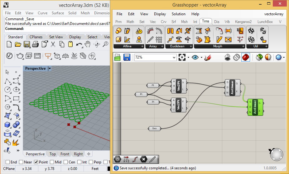
Note that a linear array of 10 circles now appears in the direction of the Y-axis in the Rhino "Perspective" window.
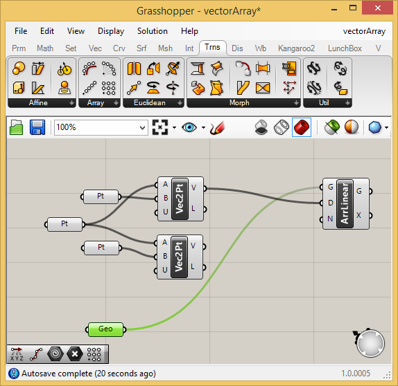
Similarly, set into place a second "AriLinear" component across to the right of the "first "AriLinear" component and accross from the second "Vec2Pt" component as illustrated in the image below. Connect the output "V" port of the second "Vec2Pt" component into the "D" (directrion) input port of the "AriLinear" component, and connect the output "G" port of the first "AriLinear" component into the "G" (geometry) input port the second "AriLinear" component. Note again that a linear array of 10 circles, one for each circle in the first array along the positive Y-Axis, now appears in the direction of the X-axis in the Rhino "Perspective" window.
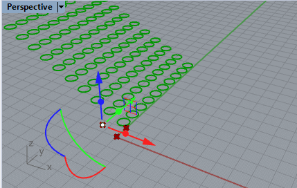
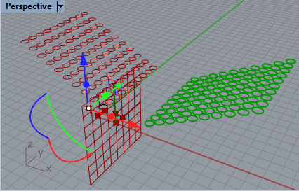
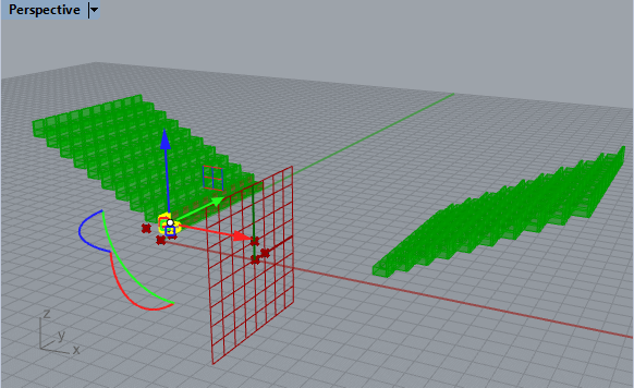
Here we've setup the vectors such that if we move the original point at (0, -1, 0) in Rhino up along the positive Z-axis we get a temporary display of inclined set of circles similar to theater seating.
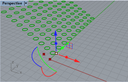
We can also move apart the circles along the direction of the Y-axis, but moving the point a (0,1,0) up along the positive Y-axis.
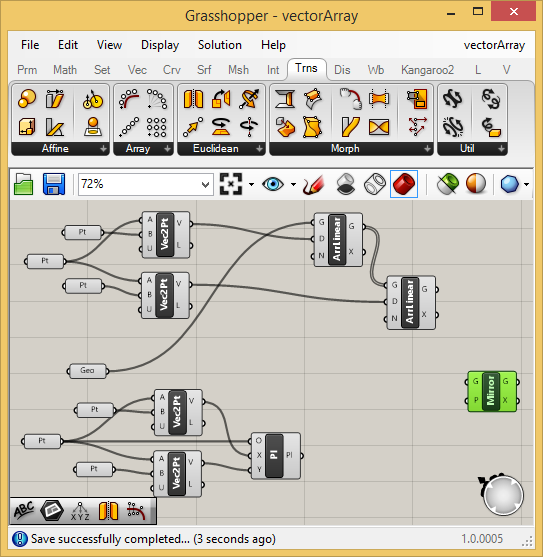
However, lets adjust the points back to their original position and work now towards mirroring the array in step 14. below.14. Mirror Array
Continuing with the same example, add three additional points In rhino at the locations (2, 1, 0), (2, 0, 0),and (2, 0, 1) as shown below. These points will form the X-axis and the Y-axis of a mirror plane.Within the Grasshopper window, add point compomponents for the point along the direction of the Y-axis (2, 1, 0), the point on the X-axis (2, 0, 0), and the point along the direction of the X-axis (2, 0, 1) similar to the beginning of step 13. Vectos and Arrays above.
To the right of the three point components, add two vector components again following a similar procedure to to the beginning of step 13. Vectors and Arrays above.
The "Pt" (2, 0, 0) component in the center at should be connected to input port "B" of both "Vec2Pt" components forming the start of each vector, and the other "Pt" components should be connected to the input port "A" of each corresponding "Vec2Pt" conponent to create a unit 1 length vector along the positive - axis and one along the Positive - axis respectively.
Within the same "Vec" tab, select the "Consruct Plane"component fom the first row second item in the area named "Plane" in the Grasshopper window , and place it to the right of the two "Vec2Pt" components the Grasshopper canvas. This new compnent is named "Pl" and highlighted in green in the canvas window below. In addtion, connect the output port "V" of the first "Vec2Pt" component to the input port "X" of the "Pl". Similarly, connect the output port "V" of the second "Vec2Pt" component to the input port "Y" of the "Pl". These two vectors establish the X any Y axis of the plane. Finally, connect the the the output port for origin point of the plane (the original point 2, 0, 0) into the input port "O" of the "Pl" component to fix it's origin at the location 2, 0, 0) along the X-axis.
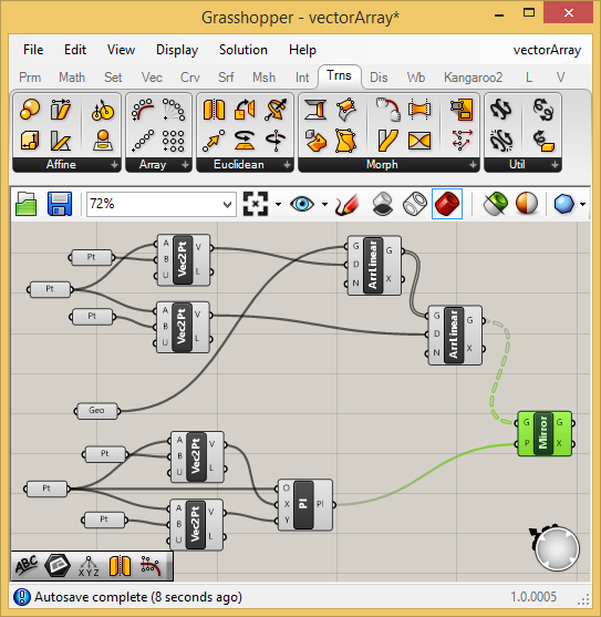
Return to the "Trns" or "T" tab in Grasshopper and in the upper left-hand corner of the area labelled "Euclidian" select the mirror component and place it to the right of bot the "AriLinear" component and to the right of the "Pl" component.To mirror the geometry of the array of circles, connect the output port "G" of the second "AirLinear" component to the input port "G" of the "Mirror" component, and connect the output port "Pl" of the "Pl" component to the input port "P" of the "Mirror" component".
This now completes the the initial Grasshopper definition for establishing the mirror of the circles.
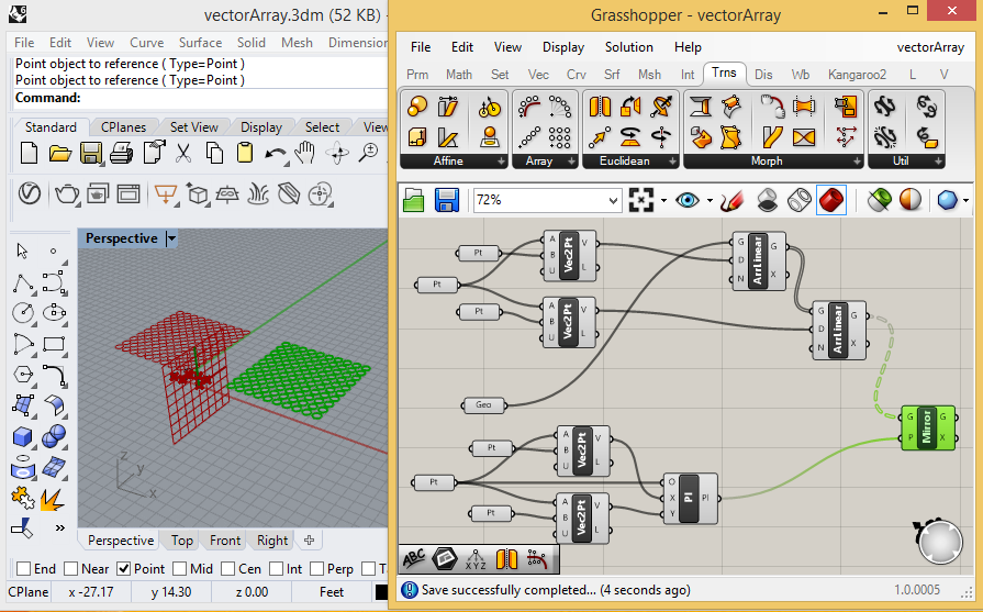
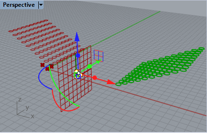
With this definition in place we can once again adjust the original points determining the vectors for the original array on the left-hand side as we did in part 13 above and the mirrored are immediately impacted. For example, the point at -1, 0, 0, and moved up the positive Z-axis, and the circles in both the original array and its mirror are inclined is depicted in the image below.
Moreover, if we move along the positive X-axis the three points that we used to construct the mirror plane, then correspoinding the mirrored geometry also moves further to the right.
15. Subsitution of geometry.
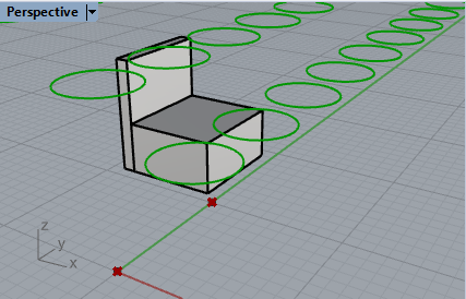
With the Grasshopper definition setup in part 14 above, it's possible to subsitute geometry for the original circle and the entire original array and its mirror are dynamically changed accordingly. For example, place a two solid boxes at the location of the original circle forming the inital array so as to create an abstract representation of a seat.
Go back to the original Grasshopper "Geo" symbol, right-click on it and then the select "Set Multiple Geoemtries" to select the two solid boxes.
The two boxes are now arrayed and mirrored in place of the original circle.Note that to add the temporary Grasshopper graphics to the Rhino model, it is necessary to right-click on the output port "G" of the second "AriLinear" component in the canvass and "bake" it, and then to do the same for the output Port "G" of the "Mirror" component.
A more static version "seating" will become a direct part of the Rhino file and separately will remain a dynamic part of the Grasshopper definition file.