Workshop 17 Notes

COMPUTER AIDED ARCHITECTURAL DESIGN
Workshop 17 Notes, Week of November 8 , 2020

SURFACES BASED UPON POLYNOMIAL EXPRESSIONS

This section picks out some polynomial expressions and the basic surfaces which they can produce.

In the examples below, polygons are described with reference to the World Coordinate System. It is an eclectic collection derived from various sources; however, there is consistency in how the basic surface elements are generated. In the examples polynomial expressions are used to calculate the vertices of a four sided facets composing the polygons. The four sided surface facets are juxtaposed in three dimensional space so as to create the larger surface areas.

A Python plugin component to Grasshopper is used in each these examples. The Python code is mostly the same in all of thes examples. The main differences are mostly confined to single polynomial expression. The Rhino file and Grasshopper file are posted to the Collab site Resources and Classes Examples folders under the folder polynomialSurfs.

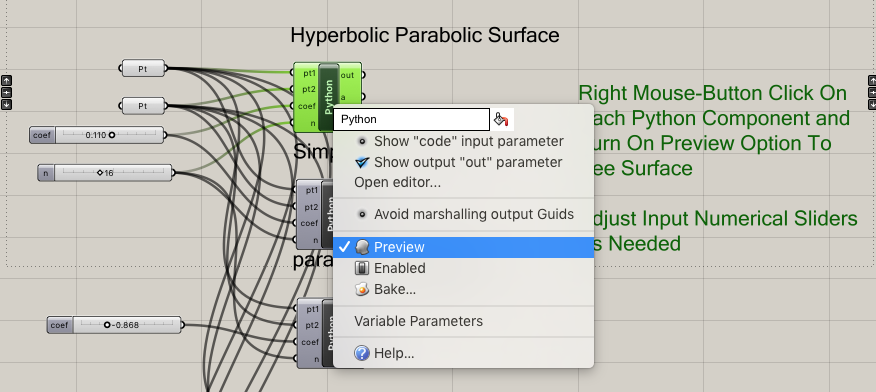
You can simply run the Python components as provided or follow the details more closely below. To activate any of the components right-mouse-button click on it and turn the Preview option as shown below.

Parts 1, 2, and 3 below provide a more detailed explanation of the Python expressions and their

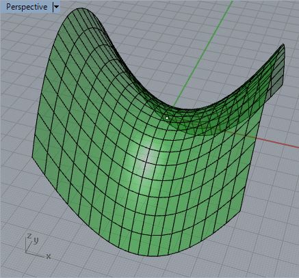
PART 1. Hyperbolic Parabolic Surface Points

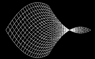
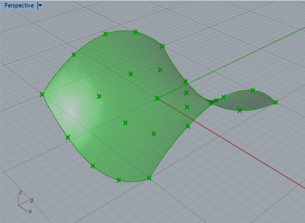
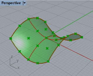
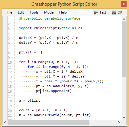
In the illustration in the figure below, we see a polygonal mesh description of a hyperbolic paraboloid shape on the left-hand side and its rendered surface description on the right-hand side [derived from Lord, The Mathematical Description of Shape and Form, John Wiley and Sons, 1984].

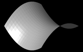Perspective View Hyperbolic Parabolic surface

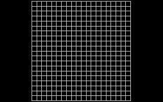
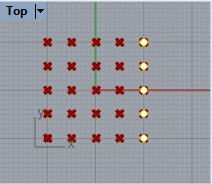
The x-coordinate and y-coordinate of the polygon vertices range over a set of values stepping in increments of 0.1 from -1 to +1. That is, we have -1 <= Point.X <= 1 and -1 <= Point.Y <= 1. Note the regularity of this uniform x-coordinate and y-coordinate grid mesh is apparent when seen in the plan view as depicted below. However, the z-coordinate changes non-uniformly from vertex to vertex and accounts most directly for the curvature that is apparent in the views of the surfaces above.

Plan View Hyperbolic Parabolic surface

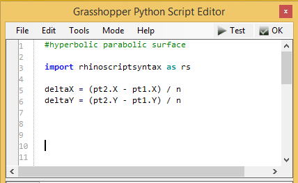
Sub procedure that calculates the z-coordinate of the hyperbolic paraboloid surface

The full Python script that generates the hyperbolic paraboloid surface will be given further below. First, however, we examine the logic of some of its parts. For each of the four sided polygons above, the z-coordinate value of each vertex is the function of its x-coordinate and y-coordinate values. The general mathematical expression used to calculate the z-coordinate of the vertices is:

z = coef * (pow(x, 2) - pow(y,2))

where s is a scalar coordinate, z is the z-coordinate, x is the x-coordinate, and y is the y-coordinate value of a particular given polygon vertex in the figure above, and where "pow" exponentiation function. Note that to generate the specific surface above, cScalar = 0.1, -10 <= x < 10, and -10 <= y <= 10. Modification of the scalar s impacts the relative height the z-coordinate each polygon vertex:

In particular, examine an expression that takes a three dimensional Point and calculates its z coordinate based on the values of each point and the scalar ccoef. That is, the expressions below take x, y, and coef, and returns a new point named newPoint with the new z coordinate as indicated below.

#calculate hyperbolic parabolic value of z for a given point on the ground plane with cordinates x and y
z = cScalar * (pow(x, 2) - pow(y, 2))
pt = rs.AddPoint(x, y, z)

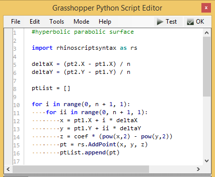
Now, we apply the hyperbolic parabolic expression for determining the z coordinate for a grid of n x n points in the ground plane that begins with a pt1 in the lower left hand corrner.

As indicated in th highlighted text box blow, the procedure begins with creating an empty list named ptList in which to place hyperbolic parabolic points. Next, we use two nested for loops, an outer loop, and indent within it, an inner loop to create a grid of 3D points.

#create an empty list of point
ptList = [ ]

#calculate the hyperbolic parabolic value of z for a grid of n x n points on the ground plane beginning with a pt1 in the lower left hand corner of the grid
for i in range(0, n + 1, 1): # iterate through each column of points in the grid
....for ii in range(0, n + 1, 1): # for each column of points iterate for n rows of points in the grid
........x = pt1.X + i * deltaX
........y = pt1.Y + ii * deltaY
........z = pt1.X + cScalar * (pow(x, 2) - pow(y, 2))
........pt = pt1.Y + rs.AddPoint(x, y, z) #use the rhinoscriptsyntax library (abbreviated "rs") to create each point
........#add the point to the point list
........ptList.append(pt)

More specifically, the outer loop expression for i in range(0, n + 1, 1) generates a set of values for i, where i = 0, i = 1, ... i = n. The expression can be interpreted as start a loop with i set to the value of 0, (0, n + 1, 1), stop the loop when i reaches the value of n + 1, (0, n + 1, 1), and for each iteration through the loop increment the value of i by 1, (0, n + 1, 1).

The outer loop stops when i reaches value of n + 1, For each such outer loop value of i, the inner loop expression for ii in range(0, n + 1, 1) generates a set of numbers ii = 0, ii = 1, ... ii = n. The inner loop stops when ii is the value of n + 1. For example, if n = 4, we get the following sequence of values for i and ii:

i = 0, ii = 0
i = 0, ii = 1
i = 0, ii = 2
i = 0, ii = 3
i = 0, ii = 4

i = 1, ii = 0
i = 1, ii = 1
i = 1, ii = 2
i = 1, ii = 3
i = 1, ii = 4

i = 2, ii = 0
i = 2, ii = 1
i = 2, ii = 2
i = 2, ii = 3
i = 2, ii = 4

i = 3, ii = 0
i = 3, ii = 1
i = 3, ii = 2
i = 3, ii = 4
i = 3, ii = 5

If pt1 is located at -1, -1, 0, coef = 0.5, n = 4, deltaX = 0.5 and delta Y =0.5, then we would get the x, y, z values for 20 points appearing in the plan view as follows:

OUTER LOOP 0 (first column of points in grid) index i = 0 , index ii = 0 -> x = -1.0, y = -1.0, z = 0.0 index i = 0 , index ii = 1 -> x = -1.0, y = -0.5, z = 0.375 index i = 0 , index ii = 2 -> x = -1.0, y = 0.0, z = 0.5 index i = 0 , index ii = 3 -> x = -1.0, y = 0.5, z = 0.375 index i = 0 , index ii = 4 -> x = -1.0, y = 1.0, z = 0.0
OUTER LOOP 1 (second column of points in grid) index i = 1 , index ii = 0 -> x = -0.5, y = -1.0, z = -0.375 index i = 1 , index ii = 1 -> x = -0.5, y = -0.5, z = 0.0 index i = 1 , index ii = 2 -> x = -0.5, y = 0.0, z = 0.125 index i = 1 , index ii = 3 -> x = -0.5, y = 0.5, z = 0.0 index i = 1 , index ii = 4 -> x = -0.5, y = 1.0, z = -0.375
OUTER LOOP 2 (third column of points in grid) index i = 2 , index ii = 0 -> x = 0.0, y = -1.0, z = -0.5 index i = 2 , index ii = 1 -> x = 0.0, y = -0.5, z = -0.125 index i = 2 , index ii = 2 -> x = 0.0, y = 0.0, z = 0.0 index i = 2 , index ii = 3 -> x = 0.0, y = 0.5, z = -0.125 index i = 2 , index ii = 4 -> x = 0.0, y = 1.0, z = -0.5
OUTER LOOP 3 (fourth column of points in grid) index i = 3 , index ii = 0 -> x = 0.5, y = -1.0, z = -0.375 index i = 3 , index ii = 1 -> x = 0.5, y = -0.5, z = 0.0 index i = 3 , index ii = 2 -> x = 0.5, y = 0.0, z = 0.125 index i = 3 , index ii = 3 -> x = 0.5, y = 0.5, z = 0.0 index i = 3 , index ii = 4 -> x = 0.5, y = 1.0, z = -0.375
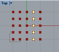OUTER LOOP 4 (fifth column of points g grid) index i = 4 , index ii = 0 -> x = 1.0, y = -1.0, z = 0.0 index i = 4 , index ii = 1 -> x = 1.0, y = -0.5, z = 0.375 index i = 4 , index ii = 2 -> x = 1.0, y = 0.0, z = 0.5 index i = 4 , index ii = 3 -> x = 1.0, y = 0.5, z = 0.375 index i = 4 , index ii = 4 -> x = 1.0, y = 1.0, z = 0.0

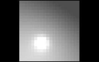
And, aswill be described in PART 2, if we were able to build the resulting hyperbolic parabolic surface for the given set of x, y, z values it would appear as illustrated below.

hyperbolic parabola based on 5 x 5 grid
Hyperbolic Parabolic Surface Based on 20 Points.

PART 2: Generating the Hyperbolic Paraboloid Surface From The 3D Points

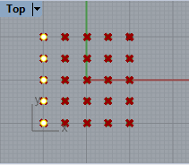
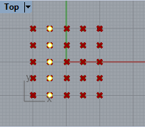
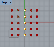
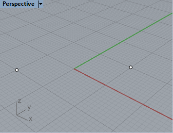
To complete the implementation the hyperbolic parabolic surface, begin by placing corner points on the x-y ground plane in Rhino at the location -1, -1, 0 and the location 1, 1, 0.

corner pts

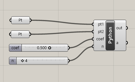
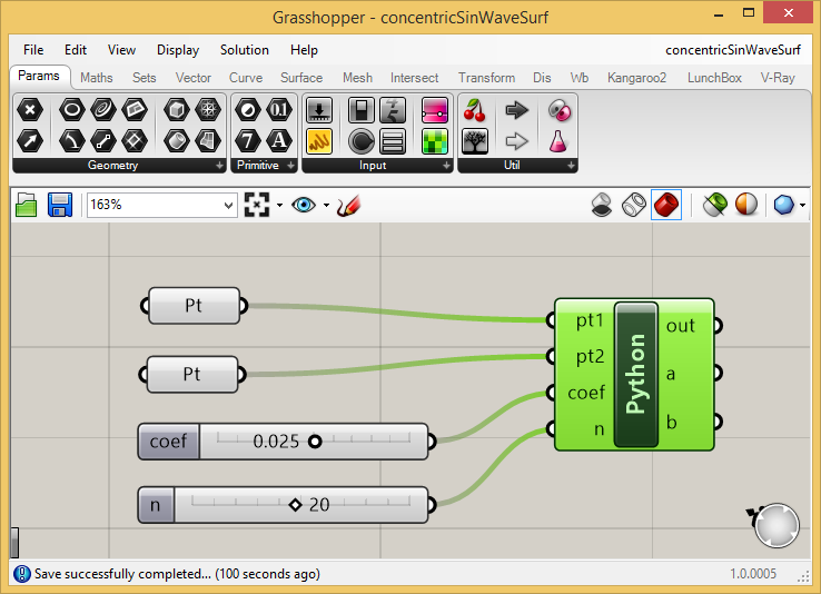
Next, as depicted in the figure below, within Grasshopper we initiate a setup by creating two corresponding "pt" components and two "number sliders".

setup canvas window

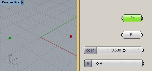
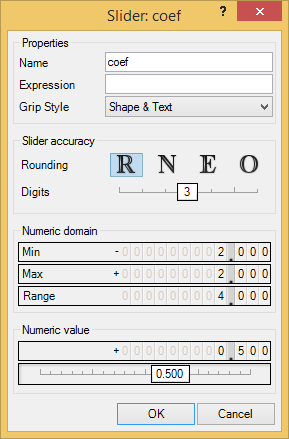
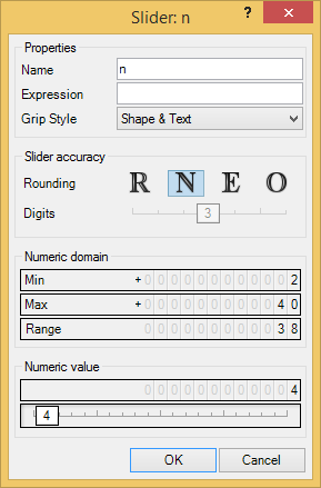
The slider named "coef" ranges in floating point coeficient values from -2.0, to 2.0 fto control the vertical scale of the hyperbolic parabolic surface, and the second slider named "n" ranges in number of surface division integer values from 2. to 40.

As depicted in the next figure below, create a Python component with two "point3d" inputs, a "float" input and an 'int" input similar to previous workshop notes, and then connect the corresponding parameters from the left side of the canvas window.

add python component

.

Add a output vaiable "b" parameter to the Python component by zooming up close and selecting the "+" symbol similar to previous workshops.

add output variable "b"

Enter the Python component. Begin editing by importing the rhinoscirptsyntax library on line 4 similar to prior workshops. We also determine the incremental distance between grid points in the x and y axis by adding variables deltaX and deltaY, where deltaX is the overall distance in the x drection divided by input variable n and deltaY is the overall distance in the y drection divided by input variable n.

initial Python script

Continuing within the script editor, add the double nested loop described in Part I above as depicted lines 8 through 16 in the figure below.

add nest loop

Continuing within the script editor, we set the output variable "a" to the pointList as depicted in line 18 in the figure below.

addpoint list output to variable a

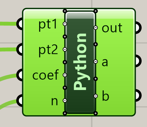
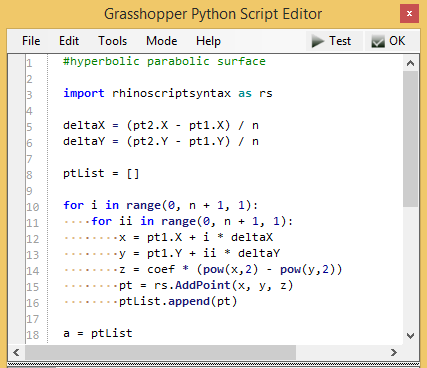
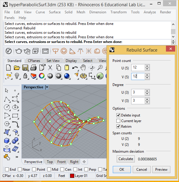
Finally, add the rhinoscriptsyntax function AddSrfPtGrid as illustrated in lines 20 and 21 below. In line 20, we create a list named "count" which containts two elements, the count of points in the x direction and the count of points in the y direction. In turn, the AddSrfPtGrid function has two inputs, 1. the count of points in X and Y direction, and 2. the ptList itself. The surface in turn is assigned to the output vaiable b.

add grid surface to script

Baking the surface yields the following result inside Rhino.

baked surface

At the comment prompt, type "Rebuild" to show a higher number of vertices for clearer visualization.

rebuild surface

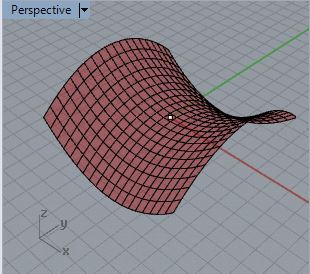
A Grasshopper file with the Phython compnent can be also downloaded from hyperbolicParabolic.gh for a hypbolic parabolic surface, It can also be easily modified to obtain most of the the variations below from "Hyperbolic Parabolic Mesh" to "Sine Surface in X and Y".

PART 3: Surface Examples Created by Varying the Input Parameters

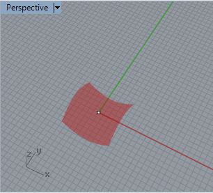
1. With the script setup in step 2, placing the corner pts at -10, -10, 0 and 10, 10, 0, adjusting the coeficient to 0.1, and baking the output , yields a similar result at a greater plan dimrension.

hyperbolic parabolic mesh

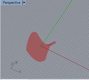
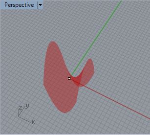
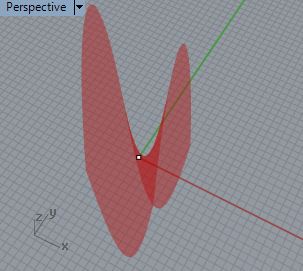
2. Varying the coeficient parameter setup gives some of the following shapes (the view has been rotated to help see the resulting geometry).


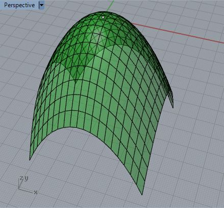
coef = 0.1	coef = 0.25	coef = 0.5	cScalar =1

PART 3. Subsituting Alternative Polynomial Expressions

1. The key to the shape of the polygon mesh in the function hyperbolicParabolic is the expression z = cScalar * (pow(x, 2) - pow(y, 2)). If we replace this function with one containing alternative values of z, it results in the following table.Note that for the hyperbolic parabolic mesh, the eliptical parabolic mesh, and the simple saddle shape, the width and height variables should be set to no greater than 10, and coef no greater than -1 to 1. For the sine function shapes, the width and depth should be no less than 360 feet, coef should be set to a minimum of 30, and numRows and numCols both be set to 100.

#Hyperbolic Parabolic Mesh z = coef * (pow(x, 2) - pow(y, 2))
#Eliptical Parabolic Mesh z = coef * (pow(x, 2) + pow(y, 2))
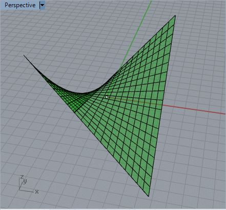
#Simple Saddle z = coef * (x * y)
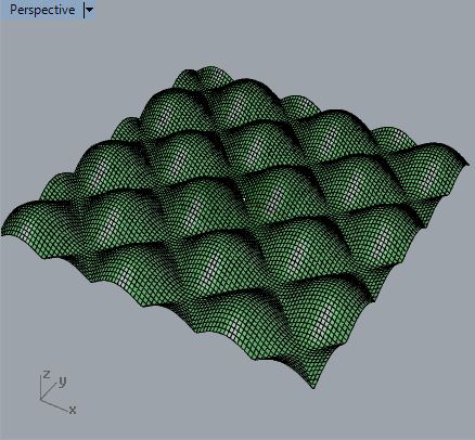
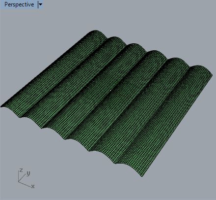#Sine Surface #Note: add the math library at the top of the script allows access the trignometry functions import math frequency = 2 z = coef * abs(math.sin(math.radians(x * frequency)))
#Sine Surface in X and Y frequency = 2 z = coef * abs(math.sin(math.radians(x * frequency)) + math.sin(math.radians(y * frequency)))
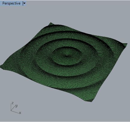
#Concentric Sine Wave dist = math.sqrt(pow(x,2) + pow(y,2)) frequency = 3 z = coef * abs(math.sin(math.radians(frequency * dist)))

In the last three examples the size of the plan is relative to the frequency of applying the sin or cos function relative to the given scale. For example, we can rewrite the scipt and adjust the parameters as follows if the corner points are still located at -1, -1, 0 and 1, 1, 0. The values of coef = 0.025 and of n = 20.

adjust coef and n

Within the script itself add the math library in line 4 and then setup for the trignometic functions in lines 15 through 17

concentric sin wave script

The baked result in Rhino concentrates the sine waves in the area delimited by the corner points -1, -1, 0 and 1, 1, 0 and when rebuilt with a 50 x 50 point count appears as follows:

concerntric sin wave

The Grasshopper file with the Python component for the concentric sine wave also can be downloaded from ConcentricSinWavSurf.gh.

Summary

Within this workshop we have developed a few basic scripts for representing three-dimensional surfaces . The principal building block of these surface elements has been various kinds of polynomial based surfaces. The examples also demonstrate the power of encapsulating the basic parameters of a particular architectural composition within a few variables. In the case of polynomial related surfaces, we were able to succinctly describe the range of the surface between two coner points, the scale of its curvature (i.e., the variable coef) and the resolution of its curvature (i.e., the variable n).