COMPUTER
AIDED
ARCHITECTURAL DESIGN
Workshop 15 Notes,
Week of November 12, 2024
SINE WAVE SHAPE AND DIAGRID
This workshop is developed in the abstract after Shigeru Ban's Paper Palace constructed for the Hanover Expo 2000. Note that there's significantly more structural detail and elements in the original work than is covered in this tutorial. The method of geometrical reasoning and visualizaiton is interpretive in a way that is consistent with other tutorials this semester.
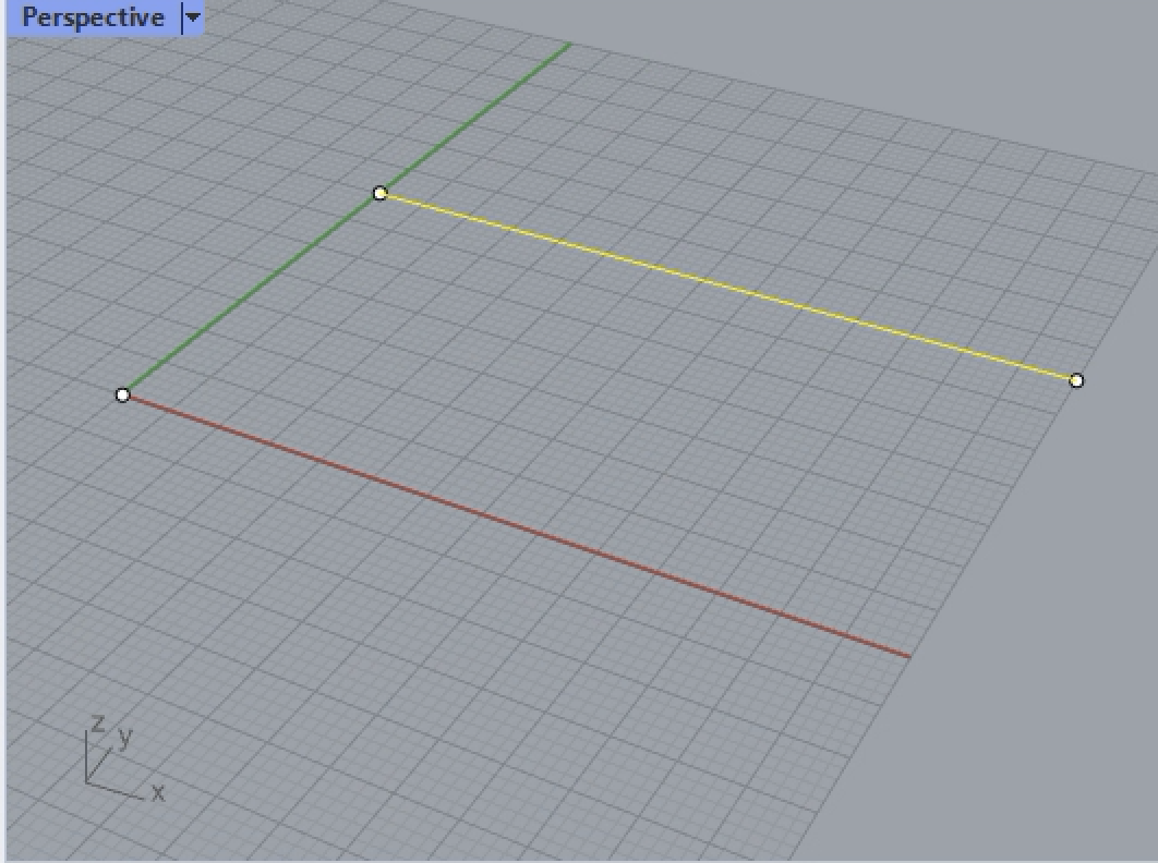
1. Initiate a Rhino drawing file at the scale of large objects feet. We begin in Rhino by creating a point at the the origin, and also a line that goes from the location 0,25 to 70,35 in the ground plane. The point will establishthe beginning of a sine curve and the line will service as an axis of bilateral symmetry.
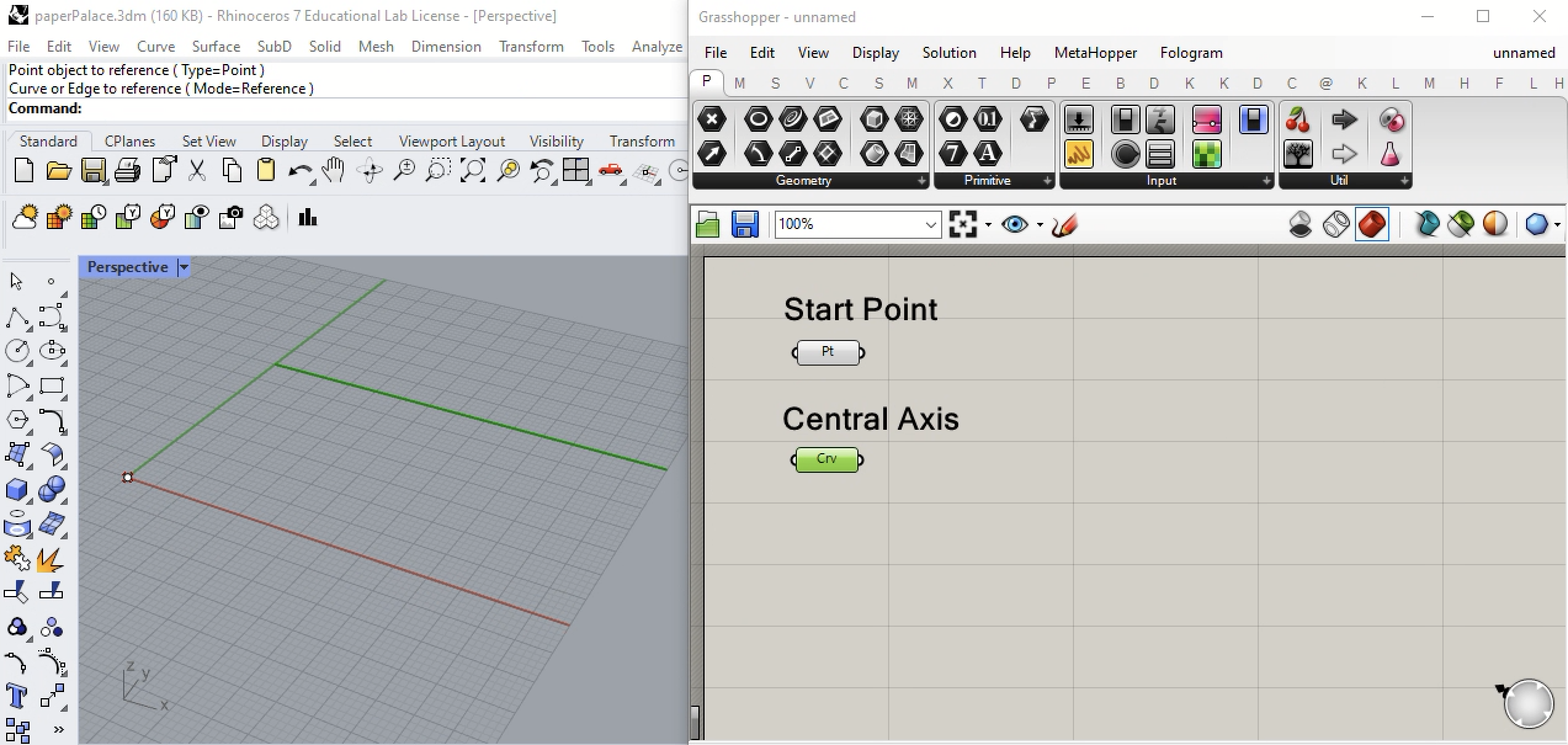
2. Open Grasshopper, go to the Prm (first) tab, initiate point and curve components in the canvas window and correspondingly select the point and axial line.
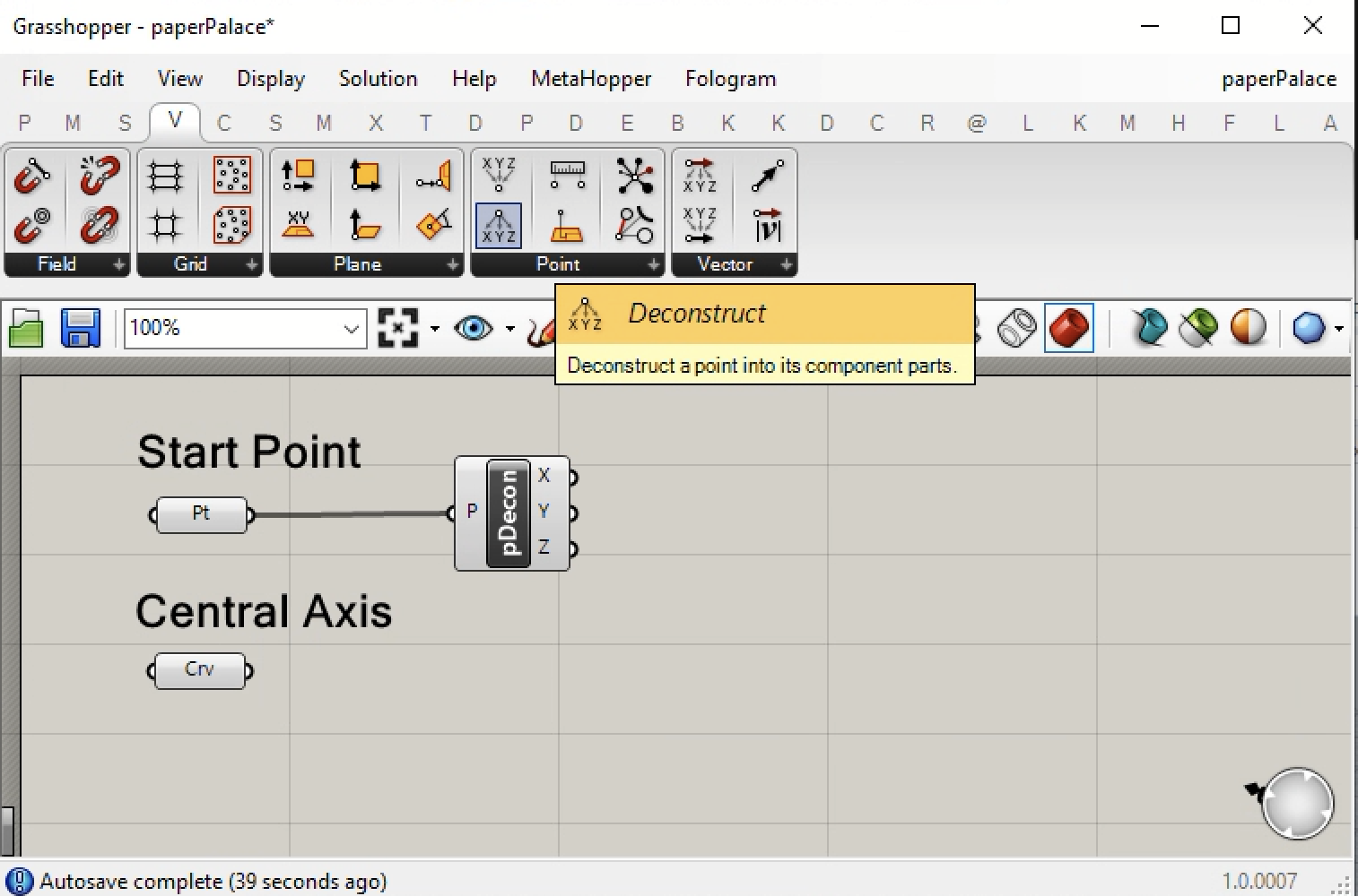
3. In the next step, go to the V (Vector) tab and select the deconstruct point icon. We will need to separate out its x componenent as a starting number for series of numbers along the x axis.
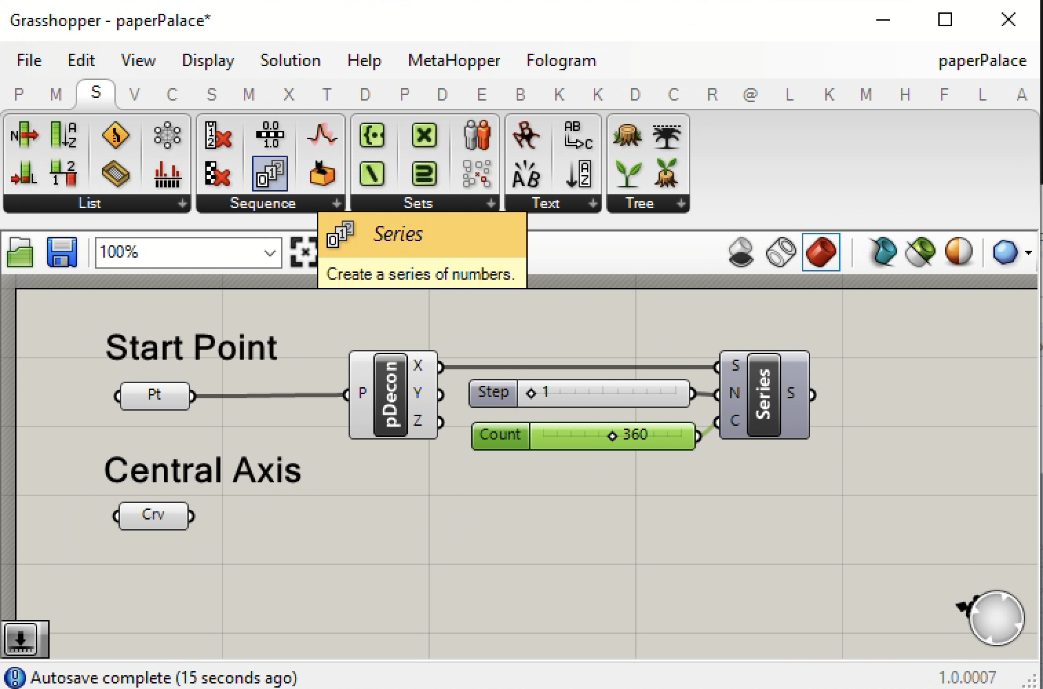
4. Now go to the S (Sets) tab, select the number Series component, and set the inputs as the x value of the start point for the input to the variable S, the value 1 as input to the variable N, and the number 360 from a number slider of 0 to 720 as input to the variable C. Here S = start number, N = step size in number sequence, and C = count of total numbers. We we use this number series to initially generate a series of degree values from 0 to 360 constitutes one full revolution around a circle. Later we will modify this number to do 270 degrees, or 3/4ths of a circle.
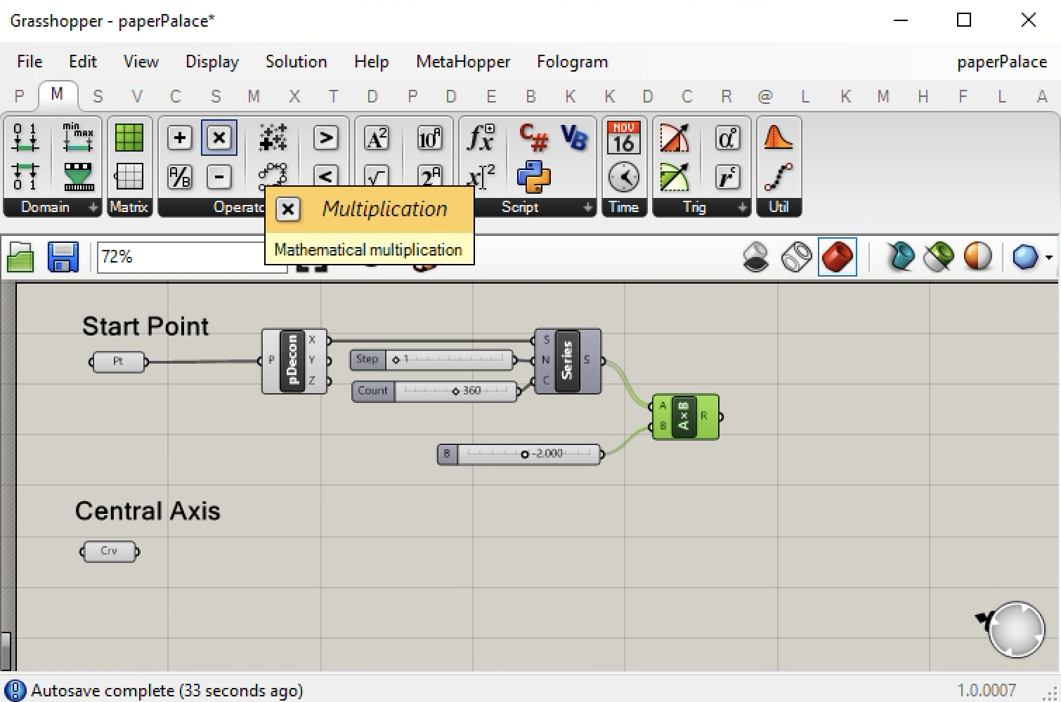
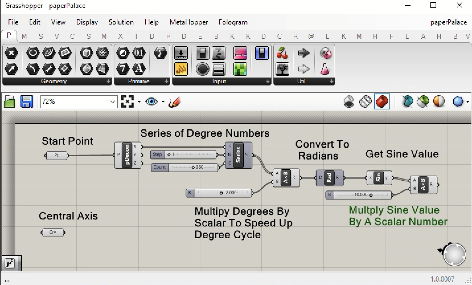
5. However, if we multiple the series of numbers output through the variable S by some other number such as -2, then instead of the number series going from 1 to 360 increasing the value of each step by the value of +1, we convert this to a number going from 0 to -720 decreasing the value the value of each step by the value of -2. This will generate a series of degrees in the negative rather than the positive direction. To achieve this result, add a number slider going from values of -30 to +30 and set the value to -2, and from the M (Math) tab, add a multiplication component. The Series output port S is connected to the input port A, and the number slider with the value of -2. is connected to the input port B.
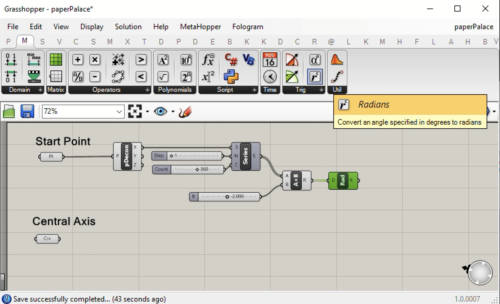
6. In order for us to apply a mathematical Sine function, we need to convert the output R of the multiplication component from degrees to radians. Thus, from the M (Math) tab, select the radians conponent and place it to the the right of the multiplication component as shown in the following figure.
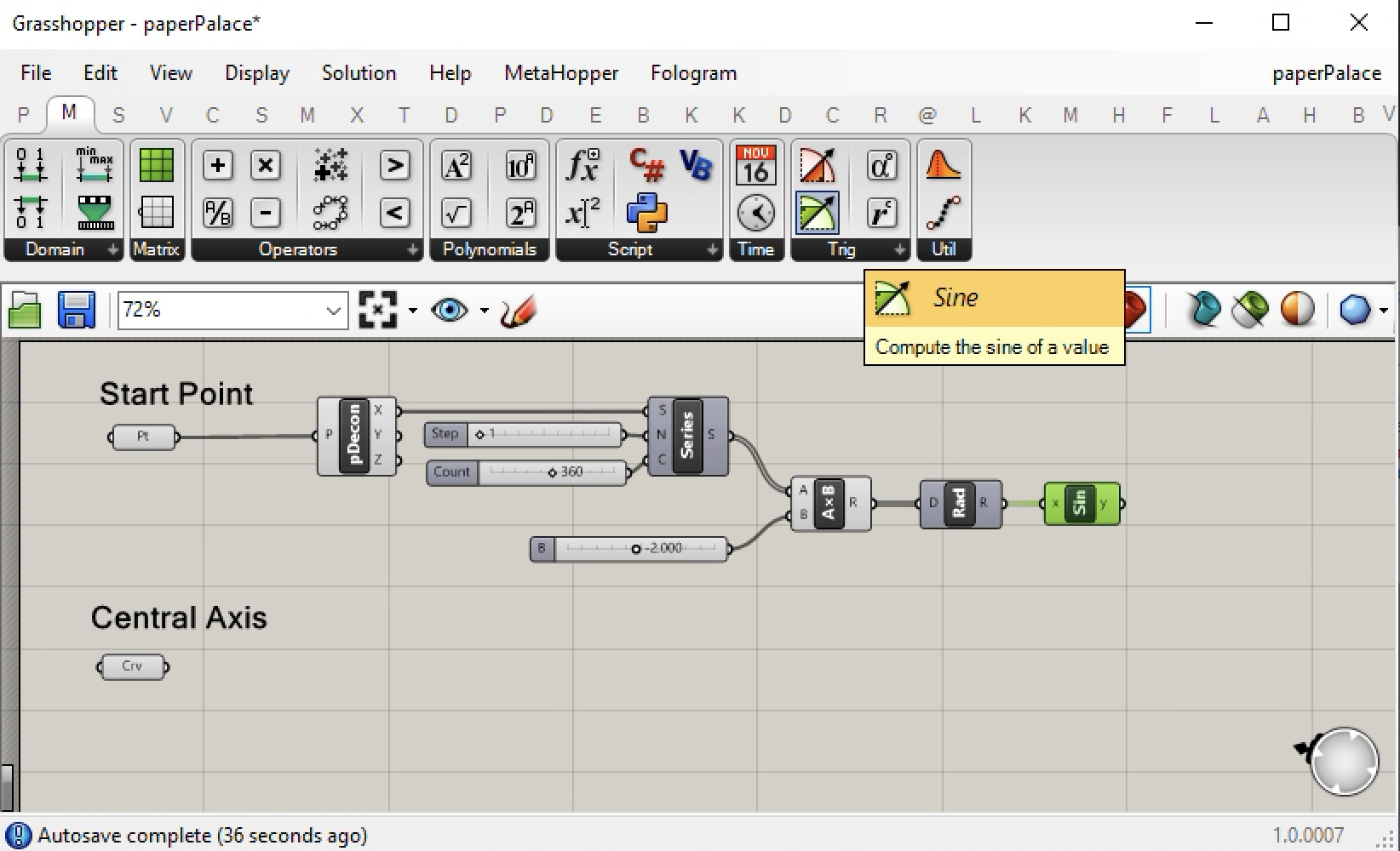
7. Now use the mathematical sine function to get the sine value of the radians as shown below with the use of the Sin component.
8. The sine function will yield values in the range of 1 to -1. However, the sine curve will need to be in value range of -10 to +10 along the y axis of the grount plane. Therefore, we add a number slider with values in the range of -30 to +30 and set the current value to 10. We than multiply the y variable output of the Sin comp by 10 as shown in the image below.
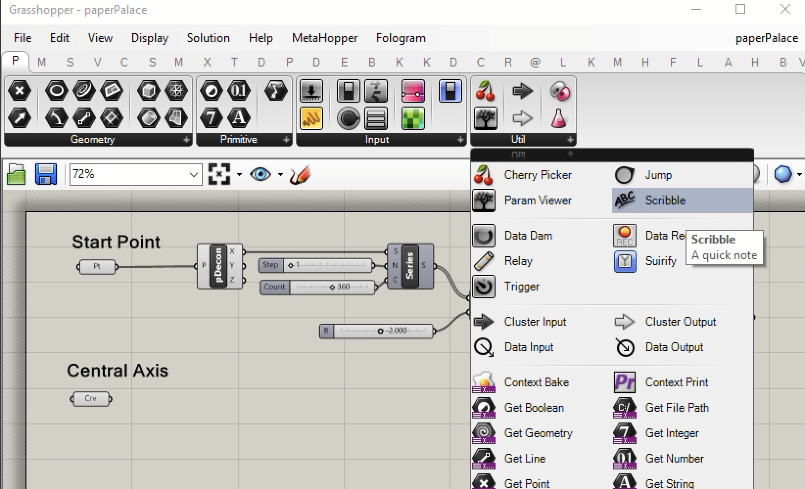
9. To clarify the steps in this sequence thus far, a few scribble notations are added to the canvas window. The scribble utility is under the P (Prm) tab, and Util panel.
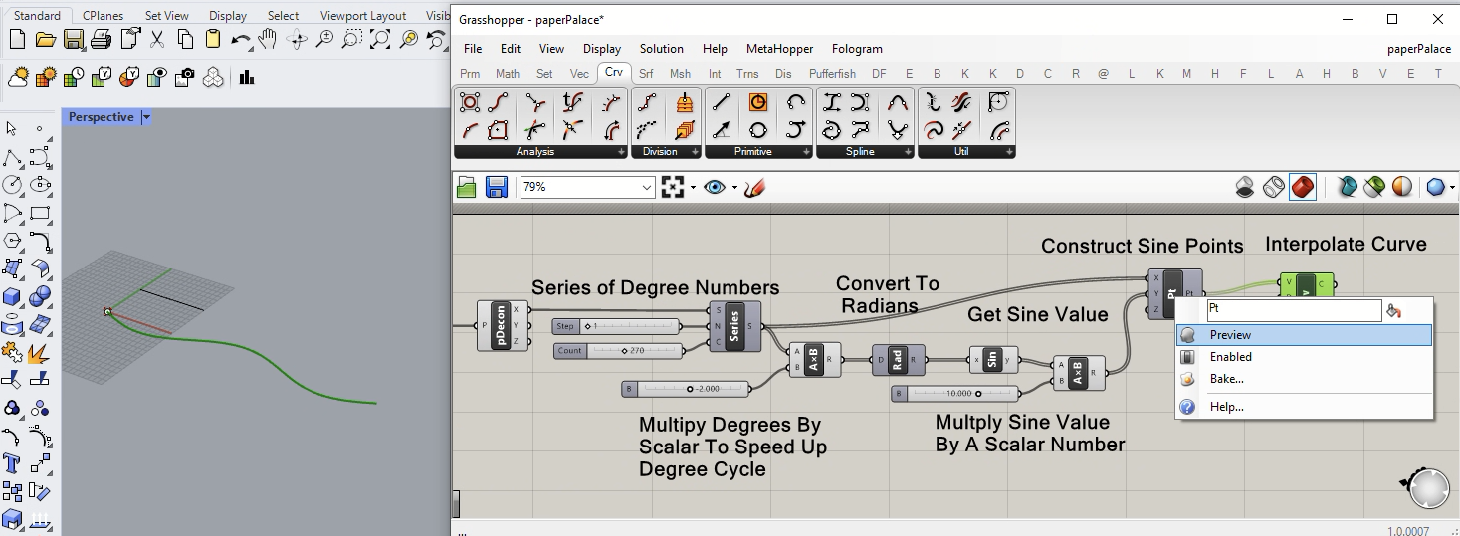
10. We can now generate a series of points forming the sine wave by going to the V (Vector) tab and using the construct point tool.
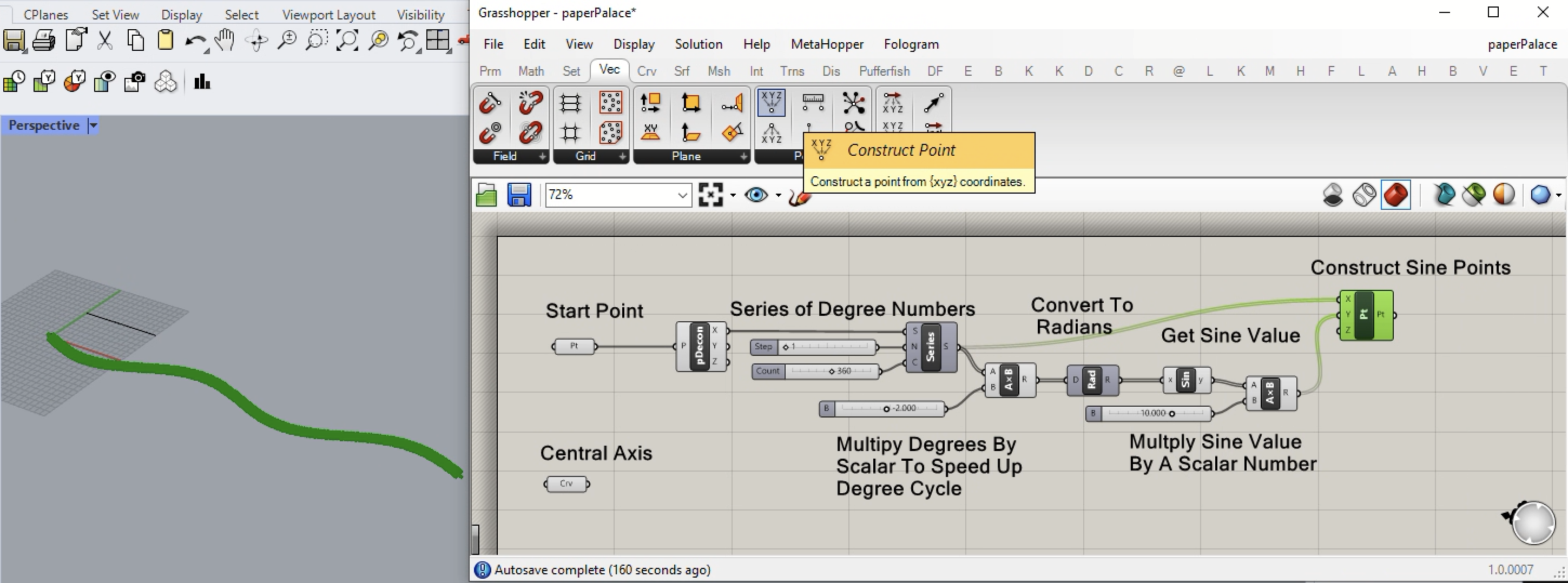
11. Note that the right-hand sine wave in the figure above begins on the left by pointing towards the + y axis direction, but concludes by pointing towards the - y axis direction. However, if we reduce the value of the Count input to the Number Series component from 360 to 270, then then both ends of the curve point in the + y axis direction.

12. In the next step, we export the series of points from the Construct Point component to the Interpolate Curve component.
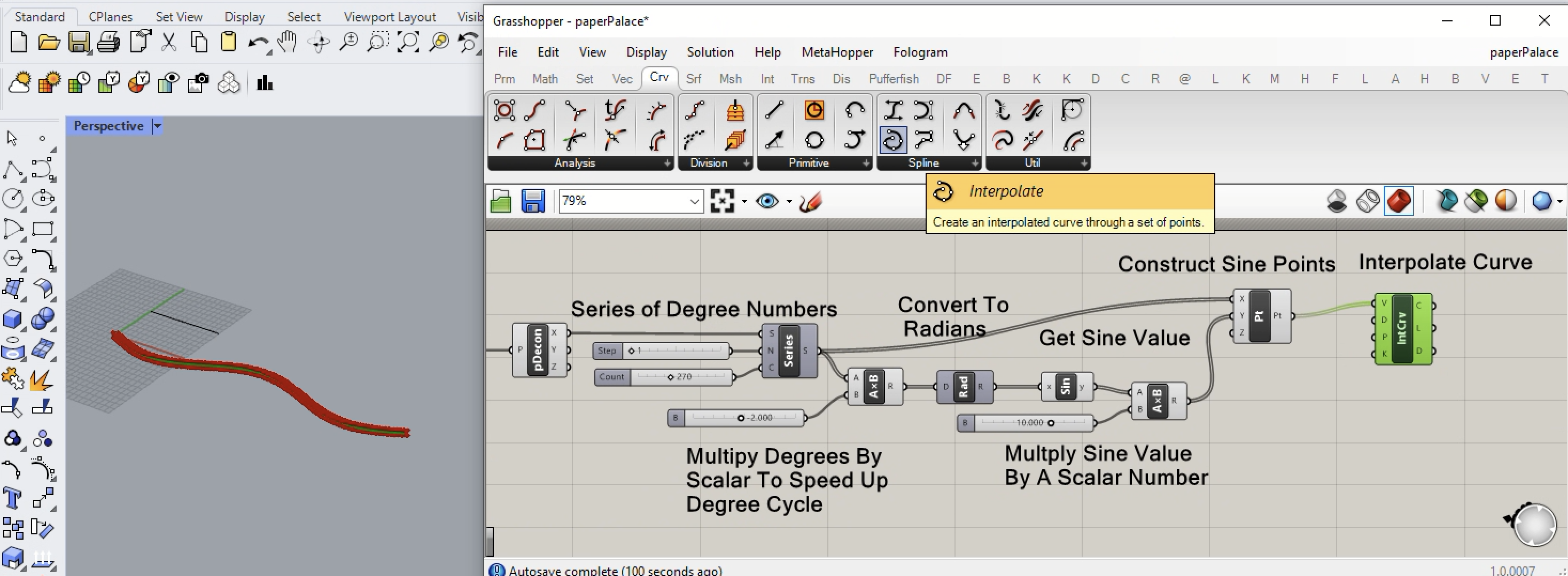
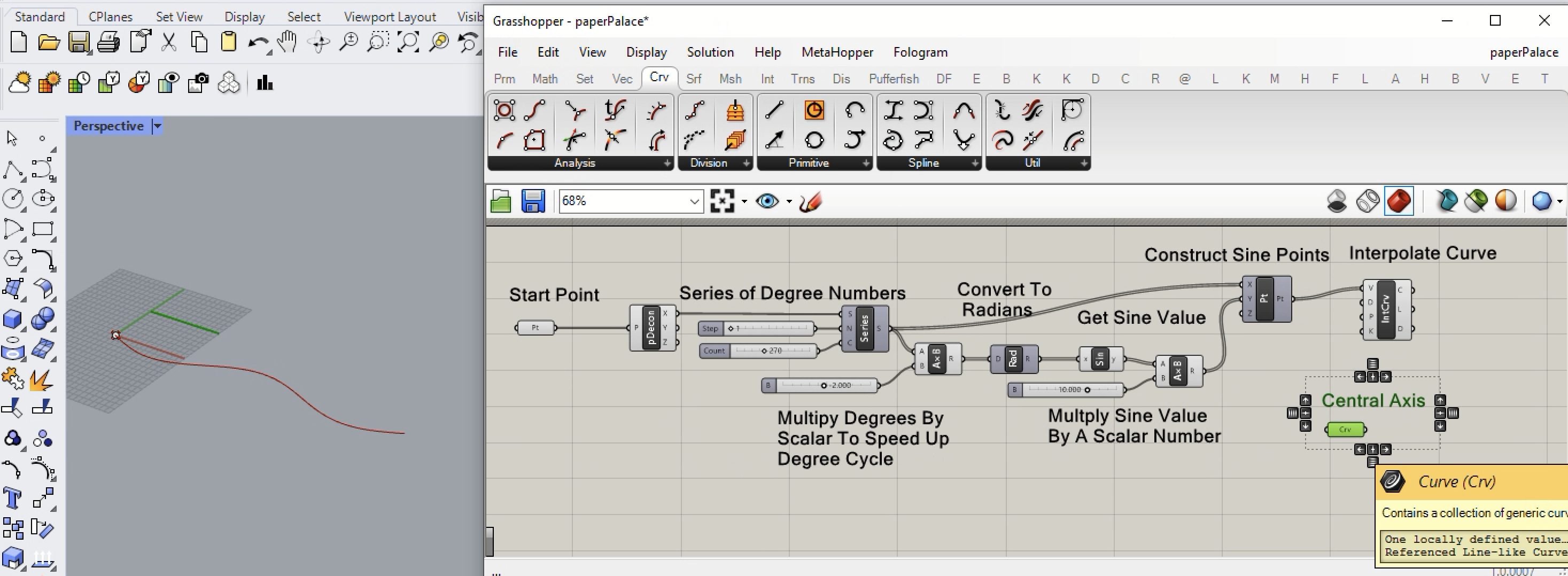
13. Turn off the display Preview opiton for the Construct Points component in order to see the curve more easily.
14. Move the central axis line component to the right side of the canvas window for more effective placement in the Grasshopper sequence.
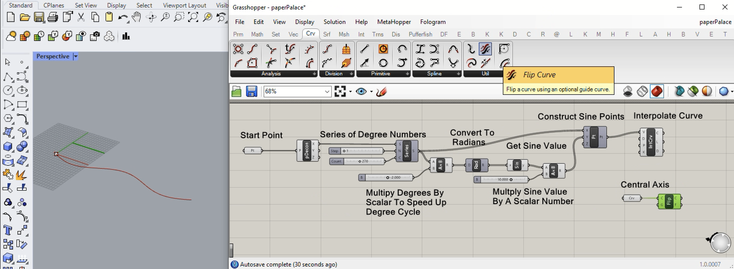
15. To setup for a surface of revolution in the next step, it's necessary to reverse the direction of the line with a Flip Curve component as indicated in the next image below.
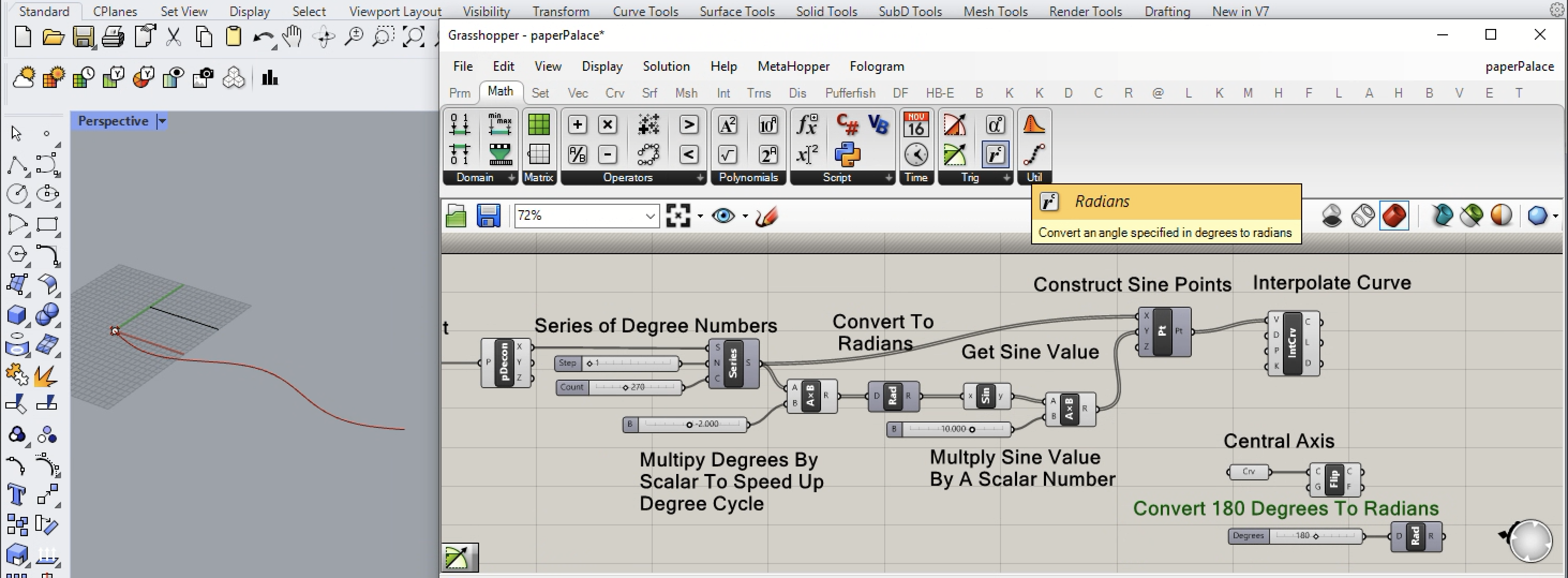
16. Next, add a number slider from 0 to 360 and set the current value to 180, and convert the value to radians.
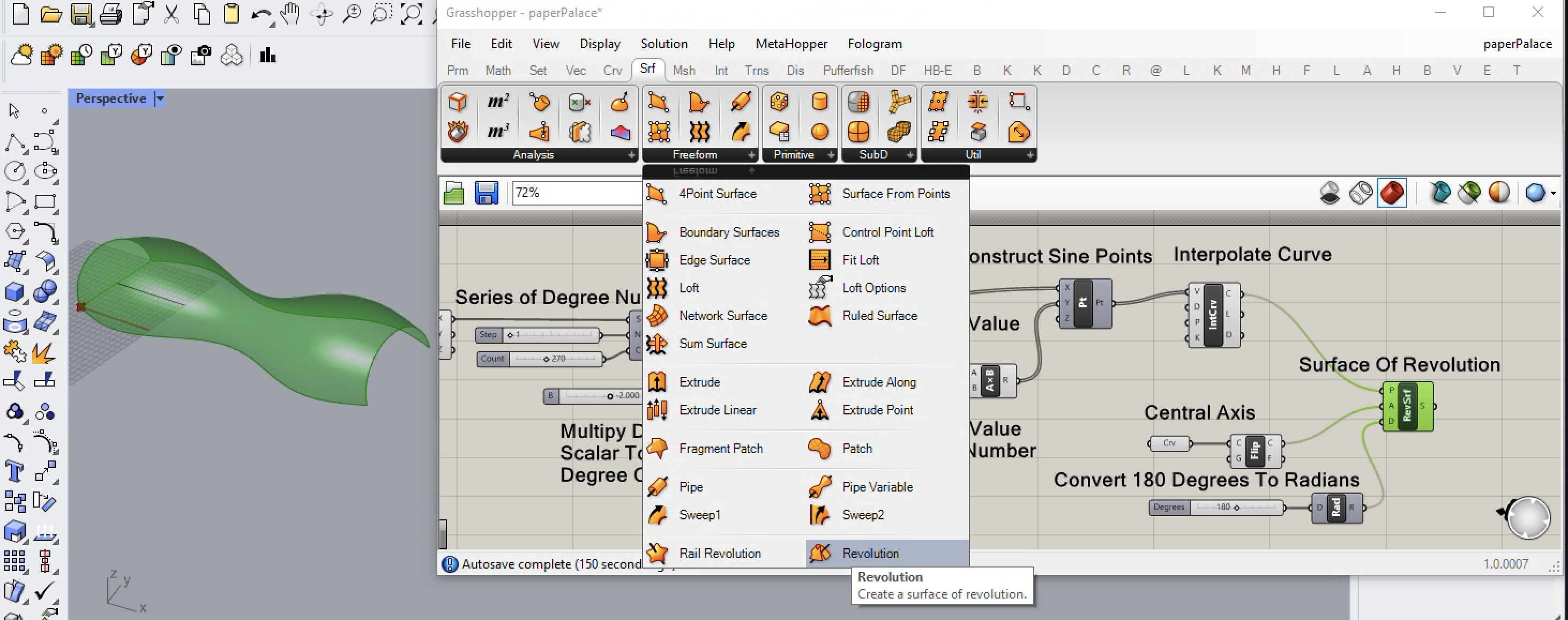
17. In the next step, go to the Srf tab and under the Freeform sub-tab, add a Surface of Revolution component to generate the roof shell of the Paper Palace. Note that the Interpolate Curve, Central Axis, and Radians of revolution are input into the Surface Of Revolution component as indicated the image below.
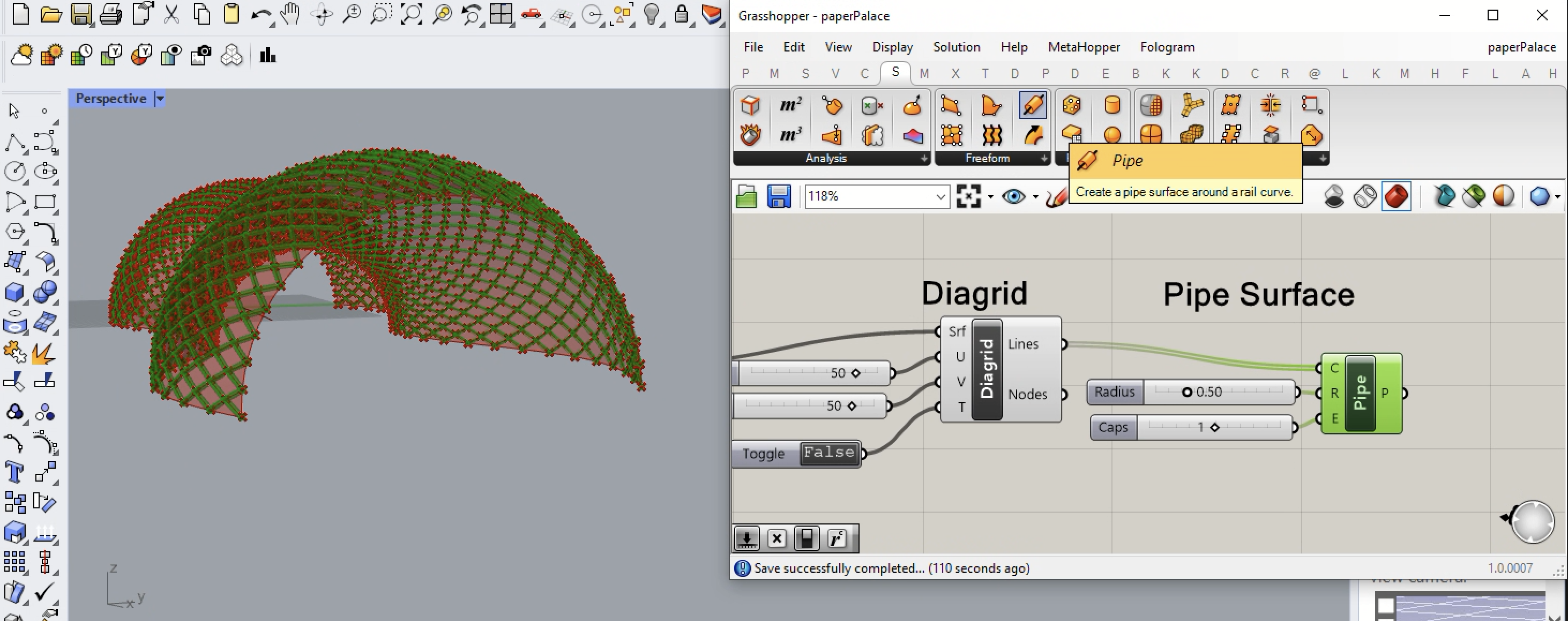
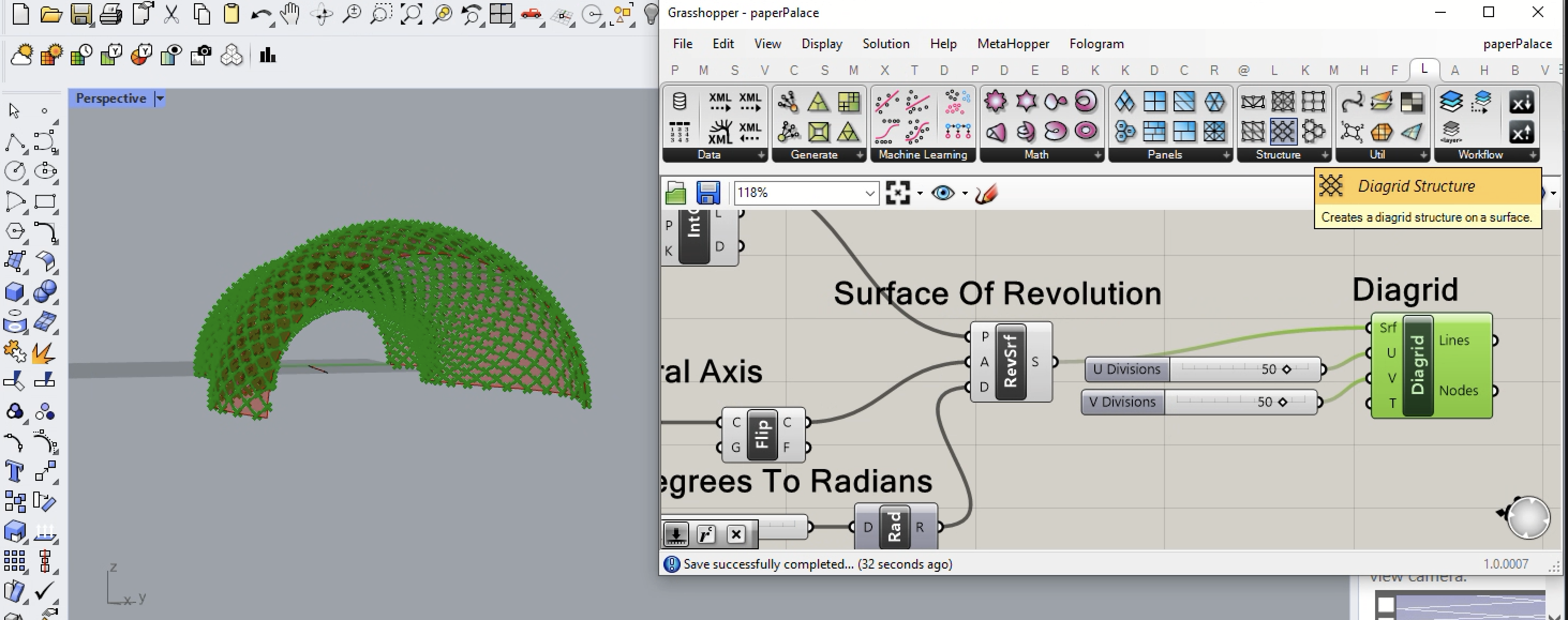
18. Go up the Lunchbox (L) plugin to Grasshopper, take the output S variable of the Surface of Revolution and input it into the S input variable diagrid component with input values for 50 each for the U and V input invariables.
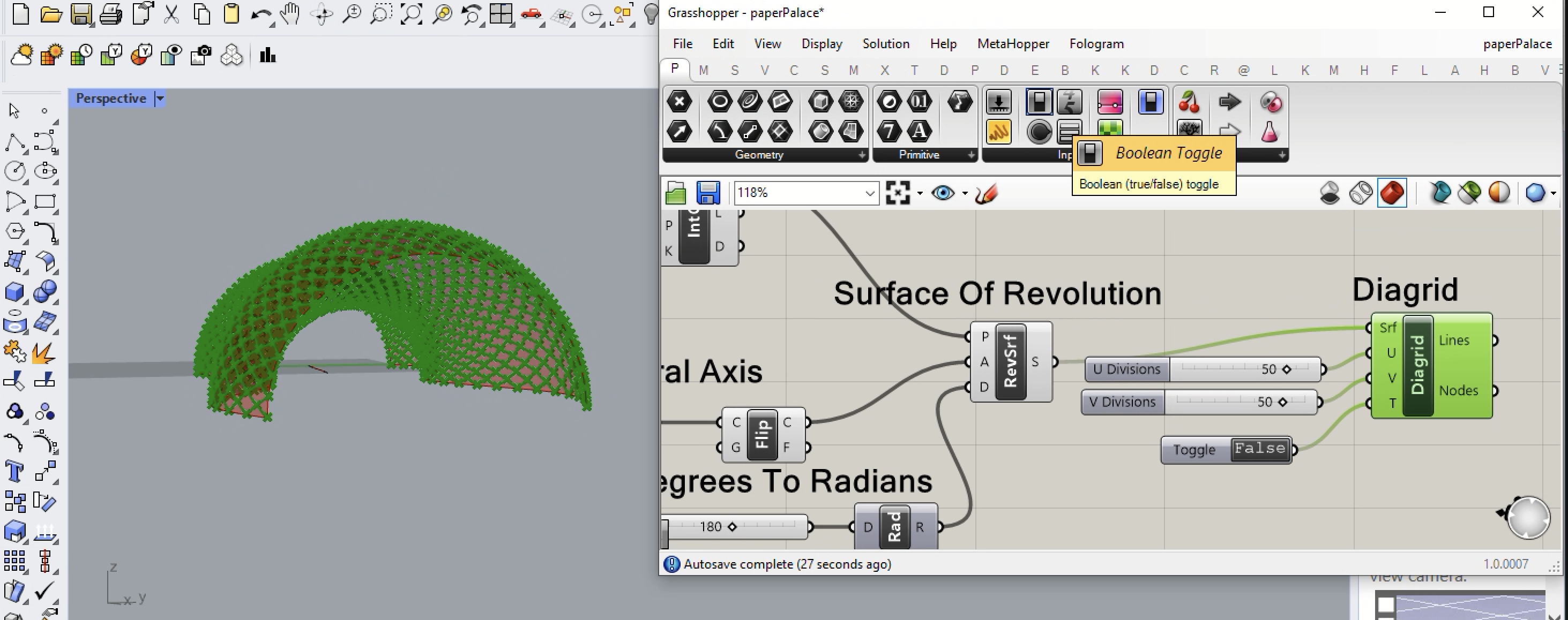
19. Returing to the Prm (P) tabl in Grasshopper, adding a Boolean Toggle to the input variable T of the Diagrid component. See below how setting the toggle to "False" shifts the placement of the diagrid relative to the corner of the surface. That is, compare the diagrid on the image below with the diagrid on the image above at the forward lower left corner of the surface.of the
20. To complete this exercise, go the Srf (S) tab and add an Pipe surface component to the right-hand side of the canvas window. In the illusration below, The input to R (radius) is set to 0.50. The input to E is set to 1 for a Flat cap at the pipe end, where 0 = No cap, 1 = Flat cap, and 2 = Round cap. For more details on pipe options, see workshop notes 13.