
| For
Internal UVa. Use Only: Draft: January 17, 2008 Copyright © 2008 by Earl Mark, University of Virginia, all rights reserved. Disclaimer |
A typical CAD system is developed with predefined data features that are useful for creating geometry. We will explore these features (e.g., points) in some detail as we progress through the chapters of this text. These predefined features allow us to build, access and modify geometry within a CAD model. They allow us to query the state of the drawing, and obtain other useful information. The system of predefined data features are used similar to the manner of the French-door example of the previous chapter. We can assign and access their data via the dot "." operator. Within this chapter we will examine their use within the context of some simple graphics programs.
We first examine the parts of a simple graphics program. We then see
how this program is implemented as a whole.
Three Dimensional Points
A predefined feature type that is fundamental to the programming of the CAD system is a three dimensional point. The point is defined with with x, y, and z components for each of its Cartesian coordinate locations. Within the GC system, a point is created with the the use of the keyword Point. We can think of a Point as having been setup with placeholders in computer memory for the following information:
|
The expression below lays out the basis for storing the Cartesian coordinate values of the point. That is, there is a placeholder for storing the value of x as a double precision floating point number (e.g., the number 1.0), and similarly y may take on the value of a double precision floating point number, and z may take on the value of double precision floating point number.
In the following expression, we initiate the variable startPoint as a specific case of the system predefined feature type Point:
| Point startPoint = new Point(); |
Once startPoint has been declared, the individual fields within it might be assigned by means of the dot ". " operator as in the following example:
| x
= 1.0; y = 1.0; z = 0.0; startPoint.ByCartesianCoordinates(baseCS, x,y,z); |
The above express for startPoint includes the arguement baseCS inside parenthesis. The name baseCS refers to the primary coordinate system of the model we are defining the point within. As we will see past this chapter, can also define points relative to alternative coordinate systems, such as one based upon the yz axis as the ground plane.
A line segment within our CAD system can be described with both a startPoint and an endPoint. For example, we might declare endPoint as follows:
| Point endPoint = new Point(); |
Once endPoint has been declared, the individual fields within it might be assigned by means of the dot ". " operator as in the following example:
| x
= 2.0; y = 3.0; z = 0.0; endPoint.ByCartesianCoordinates(baseCS, x,y,z); |
Or, we can also assign values to endPoint using our earlier startPoint as a reference location as in the following example:
| x
= startPoint.X + 2.0; y = startPoint.Y + 2.0; z = startPoint.Z ; endPoint.ByCartesianCoordinates(baseCS, x,y,z); |
The statement "startPoint.X = 2.0" is not valid, since "startPoint.X" is a read only expression in the GC language. Note that for the sake of simplifying this discussion, we are only looking at fragments of the program but not how it is organized as a whole. The relative placement of statements within a program is a key topic that we turn to in the next section. A great part of how we generate and manipulate geometry within a CAD system is based on the use of predefined data types such as Points.
Writing A Procedure
In Chapter 1, we examined how to store data on the computer through the declaration of variables of different types (i.e., integer, double, and string). In the previous section, we also looked at Point, a variable that can be used to store several values.. Now, we will explore how to use such data types within the context of a simple computer graphics program. A computer program here will be referred to as a procedure. We might think of the term procedure in terms of its everyday non-computer related use. A procedure is a sequence of instructions similar to a recipe for a cook. A procedure for making lasagna has both data and instructions.The data might consist of the raw ingredients (lasagna noodles, spinach,cottage cheese, parmesan cheese) and the instructions would consist of the steps (e.g., first lay down noodles, next lay down spinach, etc.) by which the raw ingredients are combined and baked.
Within the context of an architectural drawing, we might describe a procedure to guide someone through the steps of drawing a line starting at Cartesian Coordinate location (1,1) and extending 100 units to the right.. The architect Serlio hints at a general procedure for drawing a line in the Book of Architecture: "A line is a straight and continuous representation from one point to another, having length without width" [The Book of Architecture]. For our example of a line beginning at location (1,1), we might take off from Serlio's description the following short set of instructions:
| // Locate the
coordinates (1,1) of the starting point of the line you wish to create // Start drawing the line at (1,1) and proceed continuously // Locate the coordinates (101,1) of the end point of the line you wish to create // Stop drawing the line at (101,1) |
Within a CAD system such as GC, we might perform these instructions by hand by taking the following steps:
| // Initiate the
"PolyLine" feature // Select point (1,1) on the drawing screen with mouse and move mouse to the right continuously //Select point (101,1) on the drawing screen with the mouse for the end point of the line // Stop |
Alternatively,
we can write a procedure for the computer to more completely automate
these steps. The procedure below embeds several
kinds of statements:
(1) a non-executable comment line is preceded by
a "//" and
is used annotate what the different parts of the program do. Comment
lines are not actually executed by the procedure, but only serve to
document and clarify its processes to a person reading the text of
program itself;
(2) a declaration for point
is incorporated into a new statement,
(3) the main body of the program follows the statement "function(){",
(4) the end of the program is signaled by the symbol "}",
Note that the curly brackets "{" and "}" encapsulate the main
body of the program.
(5) instructions are sent forth to the CAD system by statements of the
form "pline1.ByVertices(verts);".
(6) These statements are then sequenced
in the example below according to the steps required for the computer to create a line. We
will become more familiar with these kinds of statements later in this
chapter.
First look at the program and its statements below. We will then
discuss the order of the statements within it:
| function ()
{ //A line is a straight and continuous representation from one point to another, having length without width //Place a diagonal line of 100 units starting at (1,1) //Initialize and save space in memory for the information related to Point features Point point1 = new Point(this); Point point2 = new Point(this); double xval, yval, zval; // Establish the coordinates of the starting point of the line you wish to create xval = 0.0; yval = 0.0; zval = 0.0; // Construct the point based upon the given coordinate values. point1.ByCartesianCoordinates(baseCS, xval, yval, zval); // Locate the coordinates of the end point of the line you wish to create xval = 100.0; yval = 100.0; zval = 0.0; // Construct the point based upon the given coordinate values. point2.ByCartesianCoordinates(baseCS, xval, yval, zval); // Create the line in GC determined by the two endpoints by selecting point1 and drawing a line continuously to point2 PolyLine verts = {}; verts = {point1, point2}; PolyLine pline1 = new PolyLine(this); pline1.ByVertices(verts); //End of Procedure } |
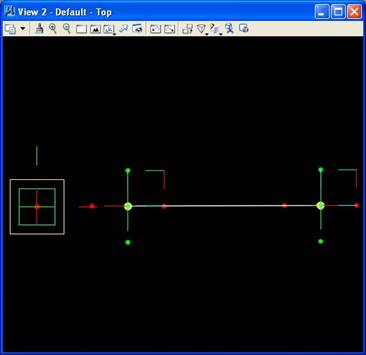
The program begins with the statement "function()". This signfies that the type of procedure, a function, incorporates no arguments since none are included inside the parenthesis "()". As we will later see, a function can act upon information passed into it through arguements. The procedure then begins to initialize features and variables, includes the statement "Point point1 = new Point(this);". This feature plays a critial role in the work of the program. As we have seen before earlier in this chapter, a Point includes x, y, and z components. The assignment statements in the program such as x = 1.0; demonstrate how the Cartesian x, y, and z values are assigned to each point. Our program draws a diagonal line from a point1 set to 1,1,0 to a point2 set to 100,100,0 (see illustration below). Thus, point1 and point2 are the primary building blocks for the database underlying the CAD model. You may note that the z-component of the two endpoints is 0.0. The fact that the z-component is set to 0.0 means that the line is a two-dimensional line in the x-y plane. We will take on three-dimensional examples later on by providing a non-zero value for the z-component.
|
Once you are familiar with the GC interface, you may run this program by downloading the following code:: |
The Macro should produce a simple diagonal line from 1,1,0 to 100,100, 0 such as illustrated below:
Analysis of A Simple Graphics Program
The structure of the simple graphics procedure above is not uncommon. As we have seen in this example they consist of the following parts within an ordered sequence of steps:
The order is very important to the successful implementation of the procedure and its step by step logic. In summary, we have established a process not unlike that of following a recipe. Some of the highlights in this preocess are that we set into place values for the first end point of the line with the expression "point1.ByCartesianCoordinates(baseCS, xval, yval, zval);", we set into place values for the second endpoint of the line with the expression "point2.ByCartesianCoordinates(baseCS, xval, yval, zval);", and we determine the line itself with statements
PolyLine
verts = {};
verts = {point1, point2};
PolyLine pline1 = new PolyLine(this);
pline1.ByVertices(verts);
Serlio's Description of Euclidean Geometry
Within Serlio's First Book On Geometry, he lays out a fundamental set of geometric elements serves to provide a foundation such that "the architect should be, if not learned in geometry, at least sufficiently knowledgeable so as to have some sort of understanding of it, particularly the general principles and also some of the more detailed matter. An abridged listing of these elements is excerpted into the table below. Rather than provide a comprehensive introduction to Euclidean geometry, it was Serlio's intention to pick the "flowers" from Euclid that might provide an architect adequate knowledge to give a good account of whatever is built. [The Book of Architecture, translation by Hart & Hicks].
| The Procedure column in the table below contains a hypertext link to a procedure in GC script. If you import the procedure into GC (e.g., right_triangle), then the figure will be generated in the active drawing window.For each example in the table below, the result will be comparable to the image at the far right. Each image at right also correspondes to a drawing in Serlio's The Book of Architecture. |
You may see the simple graphics program by selecting the program link within the table below. Review these programs for their overall order of steps and internal logic. They each rely upon the predefined data type Point as was discussed earlier in this chapter. They are simple but not necessarily efficient. Each contains more steps than really necessary to do the job at hand. They do not take advantage of certain techniques which we will explore later on. Note that they use expressions such as "pline1.ByVertices(verts);" to create graphic elements. They serve to introduce some simple graphics programs of the type we had discussed in this chapter.
| Procedure | Description | GC script | Image |
| Point | First. a point is an indivisible thing, which has in itself no dimension. | GC |  |
| Line | A line is a straight and continuous representation from one point to another, having length without width. | GC |  |
| Parallel Lines | Parallels are two lines which continue at an equal distance. | GC |  |
| Plane | A plane is made up of two equidistant lines closed off at the sides, that is a thing which has length and breadth without depth. It is also possible for planes to have different, unequal sides. | GC |  |
| Equilateral Triangle | An equilateral triangle, that is of three equal sides, occurs when three lines equal in length are joined together. This figure will make three acute angles. | GC |  |
| Right Triangle | A triangle of two equal sides occurs with two lines equal in length, that is one horizontal and the other perpendicular, and another longer line which forms the triangle. This will make one right angle and two acute angles. | GC |  |
| Triangle of Three Unequal Sides | A triangle of three unequal sides occurs when three lines of unequal length are joined together. This figure will have three acute angles | GC |  |
| Rectangle of Three Unequal Sides | A rectangle of unequal sides occurs with four lines of unequal length. This figure will have two obtuse angles. It could sometimes also have a right angle. | GC |  |
| Curvilinear bi-angular planes | Curvilinear bi-angular planes are made up of two curved, that is circular, lines. This shape will serve for many things in this book, and from it you can derive the correct normal, that is, the set square. The shape of the modern arches, which are called segmental arches, is taken from this form; and these arches can be seen upon many buildings on arched doorways and windows. | GC | 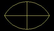 |
| Circle | The perfect circle has its centre, its circumference and its diameter. | GC | 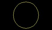 |
| Semi-circle | Semi-circle in which there is a plumb line falling upon the diameter. A right angle results from this, and it makes the half diameter. | GC | 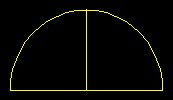 |
| Square | 'The perfect square occurs when four lines of equal length are joined together at right angles | GC | 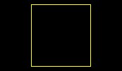 |
Serlio, having developed these basic geometric constructions, uses them in more advanced descriptions. Similarly, we will embed these basic geometric figures into more advanced compositions in later chapters of this text. For now, it is important to take note of the direct correspondence between a graphic figure and the GC procedure used to generate it. We are indebted to the early mathematicians, especially the Pythagorean, for seeing the correspondence between these parallel worlds. This link is important to computer aided design. We can setup parallel descriptions bewteen graphic figures and algebraic expressions. That is, we use a GC program to realize the creation of and modification to a drawing. Conversely, and surprisingly, we can capture the process of making a drawing by using simple CAD commands and convert it into the skeleton of GC program, at least at a fairly simple level. The following part of this chapter describes how to build a GC based procedure by capturing the steps we may use in making a drawing.
Setting up a Project
Some CAD systems have the capacity to allow you to build a prototype of a program without actually typing in any code. This approach recognizes the notion that you are in effect programming a CAD system by hand when you undertake a series of drawing commands. In particular, we could have written the simple graphics program above without having to write the text directly. We could ask the CAD system to write the program for us while we draw the diagonal line.That is, we can have the series of steps recorded and then automatically translated into a program written in the GC environment.This is a very convenient way to initialize the design of some computer graphics programs.
In this section, we prepare to build a GC program prototype through a recording of commands. Such a GC program is also referred to as a macro. We will build the prototype of a macro by using the "Point" and "Line" features to construct a drawing.
General Background
GC is an associative geometrical modeling tool that uses constraints. Geometry can be associative in the sense that the transformation of one element will be intentionally linked to the transformation of other elements. A constraint is a designed restriction on how elements may be transformed or in some specific way determines how objects may be tied together.
For a simple example, a door may be associative with an opening in a wall. The resizing of a door may be automatically linked to the resizing of the opening in a wall. The opening of a door may also have constraints with respect to the hinges which connect the door to the wall and restrict how it may move. More abstract associations between geometrical elements leads to geometrical models that are more easily changed to fit emerging directions in a design project. This first introduction of GC will demonstrate the concepts needed to construct a twisting tower. Next week, we will look at more advanced approach, where we rely more upon scripting as a way to build geometry.
Dependency Specifics of Generative Components
As alerady noted, the building blocks of a generative components model are referred to as features. Examples of features include a point, a line, an ellipse, an arc, a bspline, a surface, a polygon mesh. Points constitute one of the most basic feature types. Other types of features are defined in terms of points. For example, a line feature may be defined by two point features (end points).
Example: Line determined by two points.
A directed graph describes the dependency relationship that exists between geometrical elements. For example the coordinate system "baseCS" is the basis for the definition of two points, and, in turn, the points are the basis for the definition of a line. Within most CAD systems, these dependency relationships are somewhat hidden from the end user. Within GC these dependency relationships are more explicitly developed by and exposed to the user. Thus, the user can more self-evidently move any one of the points so as to more directly redefine the line.
Directed symbolic graph of elements.

Similarly, points can determine a bspline curve. In turn, bspline curves can determine surfaces. And, surfaces can determine the components of a paneling system. These directed relationships are defined such that changing the points can in turn propagate changes to the bsplines, and in turn, the bsplines propagate changes to the surfaces, and, again in turn, the surfaces propagate changes to the paneling systems. By exposing all the elements of this dependency hierarchy, it is easier to make dynamic changes to a computer model.
Sequence of Construction
In developing the construction of the points and line we begin by activating GC and opening the Transaction File Manager. The file manager has feature types listed such as "Arc", "BSplineCurve", etc., in the figure below. Some more commonly used feature types are also setup as icons in the top of the diaglog box, such as the one highlighted for "Create Point".
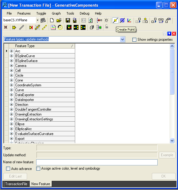
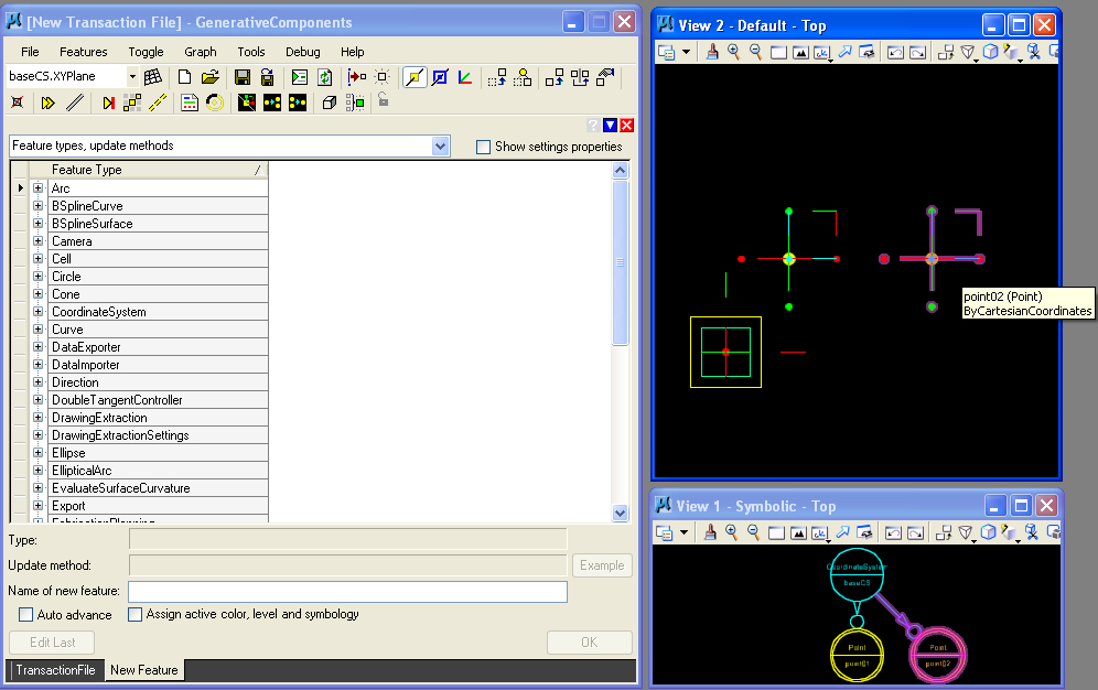
To place a Point feature in the model, you can select the icon and then enter a point location or point locations in in the "Top" view window. Here, the symbolic graph is updated as points are entered.
Adding the new point features to the model can be recorded as a "transaction" , a step within the procedure for creating this construction of a line. Select the "TransactionFile" tab, and select the green recording button at the bottom of the tab to make the recording as depicted in the image below.
![]()
Once the recording button is hit, the transaction in listed numerically and can be annotated as with the statement "Place two points in the model".
![]()
In the next step of our transactions, we return to the feature type lists by selecting the "Create Feature" button.
![]()
From the feature list, we select the "+" symbol next to the "Line" feature, revealing the expanded dialog below, Placing the mouse into the text box for "StartPoint", we can enter the name "point01" or hold down the "ctrl" key and select it from the "Top" window. Next, do the same for "point02".
![]()
Hitting the OK button for the "New Feature" results in a line being placed in the model.
![]()
This line can then be recorded as a transaction as we did in the case of the two points. Note that each transaction is recorded as a separate step thus producing a step by step macro. Note too that the "Symbolic" graph is growing, showing the dependency of the line (green symbol) on the two points (yellow symbols). By selecting the "+" symbol of the second step, we can expand the last transaction for modification of the selected points. By selecting off the green dot of this transaction, we can undo it, returning the model to the previous state that existed before the addition of the line.
![]()
In this example, the steps are dependent, and so moving a point results in changing the disposition of the line, yet another transaction if we wish to add it on to the previous two steps. In the image below, the "move" icon is selected, and the location of "point02" is changed. The line moves with it.
![]()
Returning to the "TransactionFile" tab, we can record the step of moving the line.
![]()
Further still, we have the option to "delete" or "supress" the last step, returning the line to its original postion. Thus we can revise the procedure that we've recorded making our macro very accommodating of changing expections of what is needed.
![]()
By suppressing the transaction, we retain the information related to the transaction, but undo its consequences. Thus, we preserve the history of the action for later re-use if needed. In the following image. the transaction is greyed out indicated it has been suppressed. The model has also been restored to its previous state. We can continue to modify the model adding more transactions, but leaving this last transaction suppressed or restoring it later on as needed.
![]()
In this example, we see the flexibility of the macro for handling a range of outcomes, and the possibilty to reverse steps in the construction of a model. We can go further, and be more explicit in the description of each step by using a scripting language that allows for algebraic expressions and other types of abstract expressions.
Macro Function Expressions
This last example demonstrates a procedure developed by hand. A more explicity developed procedure may rely upon the use of a "function". A function was used in the case of the diagonal line introduced at the beginning of this chapter. Now, returning to the same example, the steps required to create this function will be illustrated.
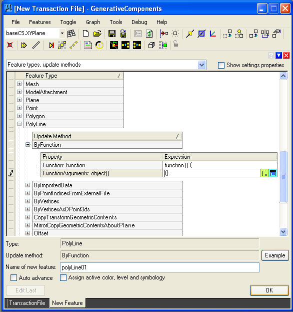
A graphical feature can be defined by referring to explicit geometry already existing in a CAD model (i.e., the points used to create the line in the preceding example). It can also be defined by the more explicit approach of writing a "function". We set out to draw a line by selecting the PolyLine feature in the Transaction File manager. Once entering into the PolyLine feature, we open the "+" symbol adjacent to the "ByFunction" method resulting in dialog box below.
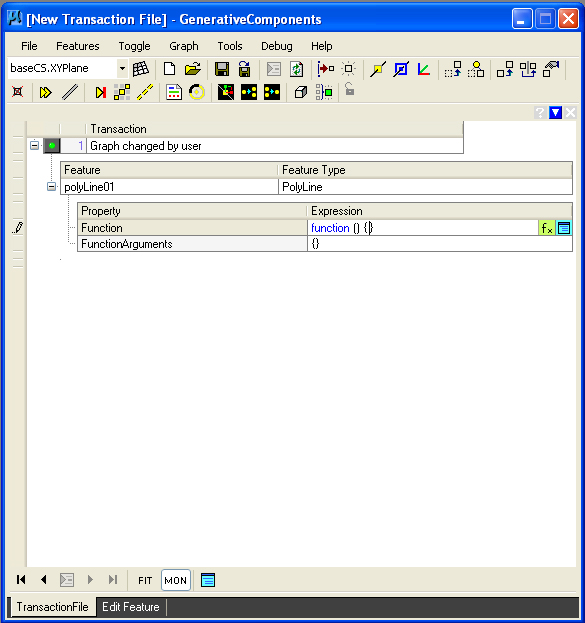
As indicated in dialog box above, we enter the expression "{}" in the "FunctionArguments" text box, highlighted in the color pink. We use the expression "{}" since this function will not have any arguements. We will examine the use of arguments in other examples.

We also enter the expression "function(){}" in the Function text box to initiate its description. Or, more directly we can select the blue-green icon at the far right of this dialog box.

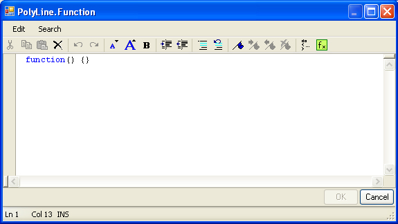
By selecting the bluee-green icon at the far right of the function text box, we enter into a function editing window "Polyline.Function". Note that the left and right parenthesis "()" on the first line of text inside the box typically contain the argument list to the function. Since there are no arguements to this particular function, then there is not any text between the two parenthesis. The two curly brackets "{ }" are to contain the main body of expressions for the function, the part to be added into this dialog box.
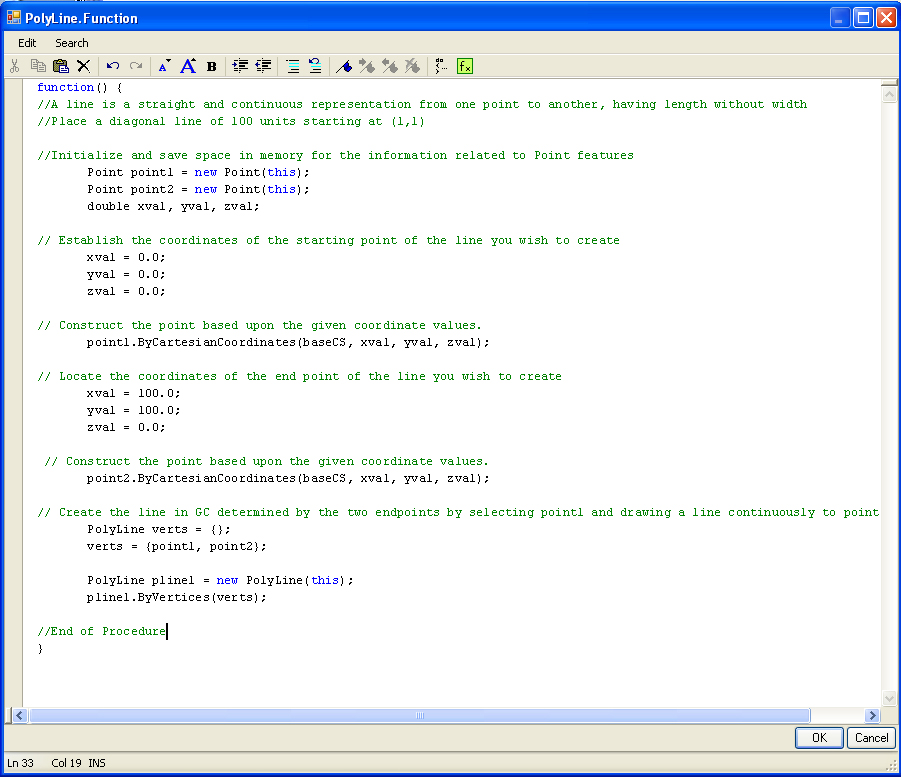
Within the Polyline.Function window, the specific procedure for drawing the dialogonal line is entered as follows, with comment lines indiced in green and preceded by a "//" symbol. The parts of this function have already been described at the beginning of this chapter.Once the full text is entered, select the "OK" button at the bottom of the dialog box to conclude use of the "Polyline.Function" dialog box..
Once the function as been described and the "OK" button selected, you are then returned to the New Feature dialog. Here, you also need to select the "OK button (bottom right of figure below), and thus complete the definition of the "PolyLine" function.
The completion of the PolyLine line function results in the drawing of the diagonal line on the screen and an update to the symbolic graph.

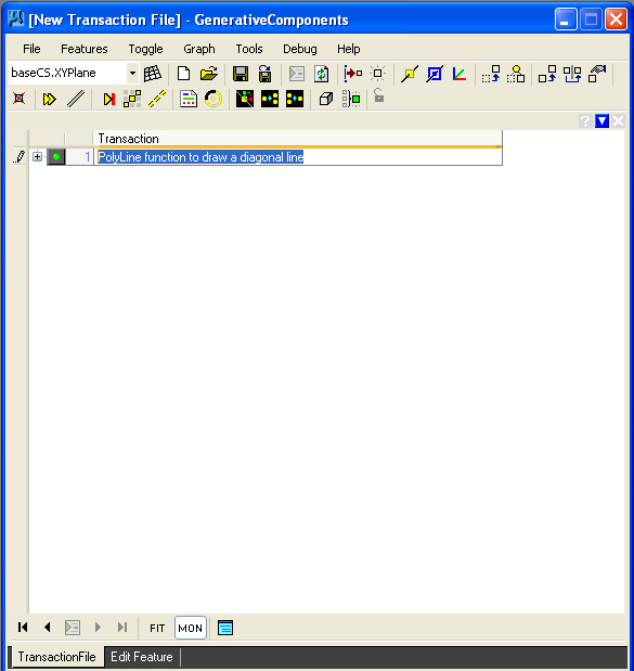
The function can then be recorded and annotated in the TransactionFile tab as we saw in the example of the two points and the line earlier in this chapter.
Arithmetic Operations
Within the example programs of this chapter, we have used the + operator for addition. TheGC scripting language has a representation for each of the other operators used in arithmetic expressions. These are summarized in the table below :
| Operator | Purpose | Number Arguments | Example | Result |
| + | addition of arguments | 2 | 1.4 + 2.0 | 3.4 |
| - | subtraction of arguments | 2 | 4.0 - 2.1 | 1.9 |
| - | negation of arguments | 1 | -5.0 | -5.0 |
| * | multiplication of arguments | 2 | 4.1 * 5.8 | 27.28 |
| / | Divide first argument by second argument | 2 | 24.9 /8.3 | 3.0 |
| \ | integer divide first argument by second argument | 2 | 5\3 | 1 |
| % | calculate integer remainder of first argument divided by second argument | 2 | 5 mod 2 | 1 |
| Pow(a, b) | raise first argument to the exponent specified by the second argument | 2 | Pow(3,2) | 9 |
The + operator is also may work on text strings, such as in the express "Archimedes "+"Spiral" which yields the concatenated expression "Archimedes Spiral". The & operator may used be used in the same way on two text expressions. Therefore, we have the string concatenation operators:
| Operator | Purpose | Number Arguments | Example | Result |
| + | concatenation of string arguments (or use to add numbers) | 2 | "Archimedes " + "Spiral" | "Archimedes Spiral" |
Several operators may be combined within a single expression. For example the expression 4 + 3 * 5 combines the addition and multiplication operators. When this is written into a GC program, the interpretation is not the same as it would be in standard algebraic interpretation. In particular, if we were to evaluate 4 + 3 * 5 in the standard way by hand, we would apply the operators from left to right. This expression would then be evaluated by first adding 4 to 3 to yield the number 7, and then multiplying the number 7 by 5 to yield the number 35. However, if the same expression of 4 + 3 * 5 were to be evaluated within a GC program, the order in which the operators are applied would be different. The computer's evaluation method would scan the expression from left to right as in the case of evaluating it by hand, but it would give precedence to some operators over other operators. That is, the evaluation still occurs from left to right, but operators with higher precedence are done first. In particular, it would give precedence to the multiplication operator * over the addition operator +. The evaluation would begin with the multiplication of 3 by 5 to yield the number 15, and then adding the number 4 to 15 to yield the number 19.
A few more expressions below give further evidence as to how the computer evaluation procedure works. Within each example, the initial line is replaced by a new line where the rules of evaluation have been applied in the correct order.
4 + 6 +
2 * 30
4 + 6 + 60 {multiplication operator is handled first
10 + 60 {result from adding 4 + 6
70 {result from adding 10 + 60
3 * 4 *
2 + 1
12 * 2 + 1 {result from multiplying 3 * 4
24 + 1 {result from multiplying 12 * 2
25 {result from adding 24 + 1
Note that parenthesis ( ) can be used to establish a precedence that overrides the normal operator precedence. We can apply parenthesis to the previous examples, and we change the results of the computer evaluations:
4 + (6
+ 2) * 30
4 + 8 * 30 {parenthesis operator is handled first
4 + 240 {result of giving the multiplication operator precedence
244 {result adding 4 + 240
3 * (4
* 2 + 1)
3 * (8 + 1){result from multiplying 4 * 2
3 * 9 {result from adding 8 + 1
27 {result from multiplying 3 * 9
All the arithmetic operators have a precedence rating. Parenthesis can be used to override the precedence ratings and sometimes make expressions more understandable. The precedence ratings for the arithmetic operators from highest to lowest are listed in the following table:
| ( ) | Parenthesis |
| - | Unary minus with one argument, e.g., -3 |
| *, / | Multiplication, Division |
| \ | Integer Division |
| Mod | Modulo |
| +, - | Addition, Subtraction |
| + | Concatenation |
Summary
Within this chapter we have introduced the graphics Cartesian coordinate system and have illustrated some simple graphics procedures.We have also drawn a parallel between some basic graphics procedures and the Euclidean "flowers" which serve to lay out the basic geometry that Serlio finds relevant to describing architectural form. We noted that the process of making a sequence of CAD commands by hand is similar to that of developing the steps within a simple graphics procedure. We further saw how a recording of the CAD commands done by hand can be translated into a prototype scripted procedure. Finally, we reviewed the set of arithmetic operators and precedence rankings by which the arithmetic operators can be evaluated. As we develop more powerful procedures in the the following chapters, we will see how a these operators can be used to describe algebraically many geometrical forms found in nature and architecture. We will also see how the parenthesis operator can be used to give these algebraic expressions clarity and simplicity.
Within the next chapter, we begin to look at recurring relationships between similar kinds elements in a graphics composition. Some of these relations can be expressed concisely as a GC scripted procedure. The conciseness comes into play where we specify in just a few expressions a seemingly large number of recurring relations that occur in a graphics composition.
Homework 2: Prototype and Modify a Script