Computables of Architectural Design: Chapter 6

WORKSHOP/SEMINAR
PARAMETRIC RAPID PROTOTYPING: Chapter 6

For Internal UVa. Use Only:
Draft: March 4, 2008
Copyright © 2008 by Earl Mark, University of Virginia, all rights reserved.
Disclaimer

Recursion and Fractals

This chapter will examine the programming technique of recursion and the related description of fractal geometry. We will first explore simple two dimensional geometries. We will then explore three dimensional fractal shapes as well as a mountain terrain.

Recursive Programming

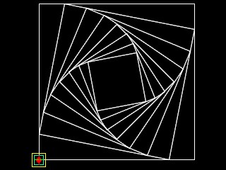
A recursive function in the simplest sense is a program that calls itself a number of times to perform parts of a task in which it is engaged. Each call of a function to itself might change the value of certain parameters thereby generating some progressive change in what is done. For example, a recursive function might describe a square that rotates inwardly at decreasing proportions. The first call of the function draws the outer most square. The next call of the function (the first time the procedure calls itself) results in the first inwardly shrinking and rotated square, as in the image of the rotating squares below. Each inner square within the progression below is determined at five sixth's times the length of the preceding outer square.

There are a total of 8 squares. Correspondingly, the recursive function is called is 8 times to perform the drawing of the square rotated at shrinking proportions. The first call of the recursive function is from the top level polygon01 procedure.

function(){
//polygon01
// Draw a series of inwardly rotating squares recursively
    Point point1 = new Point();
    Point point2 = new Point();
    Point point3 = new Point();
    Point point4 = new Point();
    Point startPoint = new Point();

    double swidth, sheight, param;
    int recur;

    swidth = 10.0;
    sheight = 10.0;
    param = 5.0 / 6.0;

    startPoint.ByCartesianCoordinates(baseCS, 0.0, 0.0, 0.0);

    point1.ByCartesianCoordinates(baseCS, startPoint.X, startPoint.Y, startPoint.Z);
    point2.ByCartesianCoordinates(baseCS, startPoint.X + swidth, startPoint.Y, startPoint.Z);
    point3.ByCartesianCoordinates(baseCS, startPoint.X + swidth, startPoint.Y + sheight, startPoint.Z);
    point4.ByCartesianCoordinates(baseCS, startPoint.X, startPoint.Y + sheight, startPoint.Z);

    recur = 8;

    //call recursive function
    drawParamSq(point1, point2, point3, point4, recur, param);

}

The recursive function drawParamSq then calls itself the remaining 7 times.

function (Point point1, Point point2, Point point3, Point point4, int recur, double param){
//drawParamSq
//Recursive program that sets up drawing the squares at parametrically determined rotatation
    Point mpoint1 = new Point();
    Point mpoint2 = new Point();
    Point mpoint3 = new Point();
    Point mpoint4 = new Point();
    //draw current square
    drawPoly({point1, point2, point3, point4});

    if (recur > 1) {
        //recursive condition
        recur = recur - 1;
        //calculate points on next square
        mpoint1 = paramPt(point1, point2, param);
        mpoint2 = paramPt(point2, point3, param);
        mpoint3 = paramPt(point3, point4, param);
        mpoint4 = paramPt(point4, point1, param);
        //recursive call
        drawParamSq(mpoint1, mpoint2, mpoint3, mpoint4, recur, param);
       } // recur == 1 implies grounding condition - recursion stops
}

The effect of the script rot_square.gct is similar to a problem for drawing a series of rotating squares that had been presented in the homework for chapter 3. The script of chapter 3 created a series of inwardly rotating squares, where each new square was sized at two thirds the size of the preceding outer square. That earlier script was written using an iterative loop.This new script, however, performs a similar task but using the technique of recursion. The recursive function drawingdrawParamSq replaces the iterative loop.

Note that the script as a whole is organized in a now familiar way with sub procedures. The utility functions are created first. The calling functions are created last according to a depency requirements, where the later functions require those addeded to the script earlier on.

Point function(Point point1, Point point2, double parameter) {
//paramPT
//find point at parameterized distance from point1 to point2
    Point returnPt = new Point();
    double xval, yval, zval;

    xval = point1.X + (parameter * (point2.X - point1.X));
    yval = point1.Y + (parameter * (point2.Y - point1.Y));
    zval = point1.Z + (parameter * (point2.Z - point1.Z));

    returnPt.ByCartesianCoordinates(baseCS, xval, yval, zval);

    return returnPt;
}

------------------------------------------------
function(Point ptList) {
//drawPoly
//draw a polygon for a given point list
    Polygon curPoly = new Polygon(this);
    curPoly.ByVertices(ptList);
}

------------------------------------------------
function (Point point1, Point point2, Point point3, Point point4, int recur, double param){
//drawParamSq
//Recursive program that sets up drawing the squares at parametrically determined rotatation
    Point mpoint1 = new Point();
    Point mpoint2 = new Point();
    Point mpoint3 = new Point();
    Point mpoint4 = new Point();
    //draw current square
    drawPoly({point1, point2, point3, point4});

    if (recur > 1) {
        //recursive condition
        recur = recur - 1;
        //calculate points on next square
        mpoint1 = paramPt(point1, point2, param);
        mpoint2 = paramPt(point2, point3, param);
        mpoint3 = paramPt(point3, point4, param);
        mpoint4 = paramPt(point4, point1, param);
//recursive call
        drawParamSq(mpoint1, mpoint2, mpoint3, mpoint4, recur, param);
       } // recur == 1 implies grounding condition - recursion stops
}

------------------------------------------------
function(){
//polygon01
// Draw a series of inwardly rotating squares recursively
    Point point1 = new Point();
    Point point2 = new Point();
    Point point3 = new Point();
    Point point4 = new Point();
    Point startPoint = new Point();

    double swidth, sheight, param;
    int recur;

    swidth = 10.0;
    sheight = 10.0;
    param = 5.0 / 6.0;

    startPoint.ByCartesianCoordinates(baseCS, 0.0, 0.0, 0.0);

    point1.ByCartesianCoordinates(baseCS, startPoint.X, startPoint.Y, startPoint.Z);
    point2.ByCartesianCoordinates(baseCS, startPoint.X + swidth, startPoint.Y, startPoint.Z);
    point3.ByCartesianCoordinates(baseCS, startPoint.X + swidth, startPoint.Y + sheight, startPoint.Z);
    point4.ByCartesianCoordinates(baseCS, startPoint.X, startPoint.Y + sheight, startPoint.Z);

    recur = 8;

    //call recursive function
    drawParamSq(point1, point2, point3, point4, recur, param);

}

There is a function drawPoly draws a square of four sides (or any closed polygon of vertices). The function paramPT finds a point located at a five sixths of the distance from a first point point1 to a second point point2. These two sub procedures are straightforward and are like those we have reviewed in previous chapters. However, the function drawParamSq is different than the functions that we have examined before, and is at the core of the recursive process. In particular, it is a function that calls itself.

The recursive process of drawParamSq is focused on two conditions.

1). The first condition is where the value of the parameter recur is greater than 1 (i.e., recur > 1). In this case the function drawParamSq will:

draw a square as determined by the points point1, point2, point3, and point4

calculate the points of the next inwardly rotated square

decrease the value of the parameter recur by one

call itself drawParamSq to draw the next inwardly rotated square

2). The alternative condition is where the value of the parameter recur is equal to the numerical value 1 (i.e., recur = 1). In this case the function drawParamSq has come to its grounding condition when the recursion itself (the process of the sub procedure calling itself) comes to a halt.

at the grounding condition, all the squares have been drawn and the process halts.

In describing this recursive function, we would identify the recursive condition as being determined by the value of the parameter recur. Recursive functions typically have a recursive condition. The recursion is typically concluded with a grounding condition (e.g., recur = 1).

Note that if the value of the input parameter recur is 8, then the function drawParamSq will be called 1 time by the polygon01 procedure, and that it will be called 7 times by the procedure drawParamSq itself. In effect, the value of the variable recur is the key to the number of recursions. The value of recur is reduced with each recursive call, leaving one fewer recursion left to perform each new time drawr56s is called.

The handling of the input parameters to drawParamSq are important to clarify with respect to the recursive process. All the point parameters are passed by value. This means that each time drawr56s is called, the value of the parameter is used in the the recursively called procedure drawParamSq. The parameter recur is also passed by value. Lets analyze them separately in the following table:

Parameters	How Passed	Analysis
point1 point2 point3 point4	by value	With each recursive call, the variable mpoint1 is created within the procedure drawParmSq. It is passed in the next call from drawParmSq. to itself through the parameter point1. Since the procedure is called recursively seven times in this example, seven different local versions of the variable mpoint1 are created with the dim statement. That is, the local point mpoint1 is being recreated with each call and doesn't impact the value of the same variable preceding the call. The same holds true for parameters mpoint2, mpoint3, mpoint4, and for point2, point3 and point4 respectively.
recur	by va;ie	With each recursive call, the variable recur is also passed by value. In each case, the passed value of the parameter recur has been decremented by 1. The program reaches the grounding condition when the value of recur has been decreased to 1. The value of the parameter recur is passed on directly, and not by going through an intermediate variable as in the case of point1 and mpoint1.

Note that recursive programming can require some sophistication in the allocation of memory for variables. This is a topic that we have avoided here. Our program is simple, but not necessarily well written for conserving memory allocation. The iteration technique discussed in chapter 3 would be much preferred with respect to conserving memory. With iteration, we re-use the same memory for variables that are re-assigned new values every time a loop is revisited.. With recursion, however, we are allocating additional memory for the re-use of the same variables (e.g., mpoint1, mpoint2, mpoint3, and mpoint4) in the recursive call. A recursive program that uses the memory management methods shown here will exhaust it more quickly than a similarly developed iterative program (i.e., it will run out of so-called stack space. a particular allocation of memory). Memory allocation and recursion is a topic, however, that we will bypass now for the sake of keeping the present introduction to recursive programming simple.

All recursive procedures could be rewritten with greater memory efficiency as iterative procedures. However, sometimes recursion becomes a more concise and expressive way to describe certain phenomenon. We will now see an example of this with the following fractal program that draws a series of triangles recursively. At the end of this chapter, we will review a procedure that based on a recursive geometrical composition, but which is developed iteratively due to memory and performance issues.

A Recursively Created Fractal

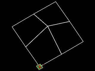
Fractal graphics have the property that the shape of its parts are self-similar to the whole. The following two illustrations of triangles, Fractal Image One and Fractal Image Two, show progressively developed examples of the same fractal. That is, the second image is a more recursive version of the first image. To understand how this is so, assume that the first image consists of a triangle that contains three smaller triangles at each of its three corners. Lets refer to each of these smaller triangles by the letter A. There is also the appearance of a fourth triangle at the center of this figure. Lets refer to this triangle at the center by the letter B. Triangle B is created as a side effect only of drawing the other three triangles A. Now imagine that we repeat the entire composition of Fractal Image One in each of its three corner triangles A. This would result in the composition of triangles at the right. Note that the fourth triangle B at the center of this figure is not changed. The second image recreates the pattern of the first image as if it reproduced a self-similar version itself in each of its three smaller triangles A.


Fractal Image One	Fractal Image Two

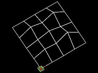
Now lets take the recursion of this pattern two steps further. Within each step, we take each of the smaller triangles A only and we repeat the entire composition of Fractal Image One inside of them. Within each step, we also do not modify the composition of Triangle B.


Fractal Image Three	Fractal Image Four

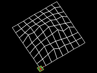
As the fractal composition progressively changes onto images five and six, the density of the triangles increase. We can still see the self-similarity of the parts of each of the progressive images to the beginning pattern.


Fractal Image Five	Fractal Image Six

It should be obvious from the study of the above images that if we were to zoom up on any part of Fractal Image Six, we would find that it contains a replication in miniature of the original composition of Fractal Image One. In the image below on the left there is a mark on an area with a red box. In the image on the right, we are given a close-up view of that red area.


Fractal Image Six With Marked Area	Fractal Image Six Close-Up of Marked Area

The script triangle_fractal.gct that generates these fractal images makes use of a recursive technique. It contains two procedures drawtri and midpt that are not unlike the geometry procedures we have examined in previous chapters. Examination of these procedures is left to the reader. Note that three graphic variables are setup to drive the script: twidth determines the width of the initial triangular side, recur is the number of recursions, and param (at 0.5) determins the division point of each triangle. It can be varied as in the rotating squares example given above. It also contains a recursive procedure drawrtri that uses a parameter recur which serves as the key to the recursive condition. This program is given below.

Note that the procedure drawRecurTri invokes three recursive calls for any value of the variable recur that is greater than 1 (i.e., recur > ).. That is, it starts three separate recursive processes for each of the three corner triangles of the original figure in Fractal Image One. The recursive process for the first corner is completed entirely before the recursive process for the second triangle is initiated. Then, the recursive process for the second corner triangle is completed entirely before the recursive process for the third corner triangle is initiated. Finally, the recursive process for the third corner triangle is performed and then we are taken to the end of all the recursions.

3D Pyramid Fractal

A 3D fractal of a pyramid works on the basis of similar principles. The animation below provides seven separate runs of the fractal drawing program. The first image is where there is no fractalization and where only a simple pyramid shape is formed. We then see in the animation the results from a number of separate runs of the program. In each of these separate runs of the program, the recursive sub procedure calls itself 1, 2, 3, 4 and then 5 times.

3D Fractal of Pyramid Through 6 Recursions

A review of the script itself reveals a logic that is very similar to the previous example of 2D triangles. The script is listed below. The sub procedures Pyramid, PpyramidPts and DrawPyramid should be easy to interpret based on the comment lines embedded within them. The main work of the program is done with the recursive sub procedure DrawrPyramid. Note that it contains a main conditional statement. Within the conditional statement, if recur = 1, then we are at the grounding condition, and a single pyramid is generated. Otherwise, if recur > 1, then five recursive procedure calls to DrawrPyramid are invoked. These five recursive procedure calls generate four recursively created pyramids in the lower four corners and one recursively created pyramid at the apex of the initial pyramid.

Point function(Point point1, Point point2, double parameter) { //paramPt //find point at parameterized distance from point1 to point2 Point returnPt = new Point(); double xval, yval, zval; xval = point1.X + (parameter * (point2.X - point1.X)); yval = point1.Y + (parameter * (point2.Y - point1.Y)); zval = point1.Z + (parameter * (point2.Z - point1.Z)); returnPt.ByCartesianCoordinates(baseCS, xval, yval, zval); return returnPt; } ------------------------- function(Point ptList) { //drawPoly //draw a polygon for a given point list Polygon curPoly = new Polygon(this); curPoly.ByVertices(ptList); } ------------------------- function(Point point1, Point point2, Point point3, Point point4, Point point5){ // drawPyramid // Draw the faces of the Pyramid Point triPoints = {}; Point sqrPoints = {}; // Base sqrPoints[0] = point1; sqrPoints[1] = point2; sqrPoints[2] = point3; sqrPoints[3] = point4; drawPoly(sqrPoints); // First Face triPoints[0] = point1; triPoints[1] = point2; triPoints[2] = point5; drawPoly(triPoints); // Second Face triPoints[0] = point2; triPoints[1] = point3; triPoints[2] = point5; drawPoly(triPoints); // Third Face triPoints[0] = point3; triPoints[1] = point4; triPoints[2] = point5; drawPoly(triPoints); // Fourth Face triPoints[0] = point4; triPoints[1] = point1; triPoints[2] = point5; drawPoly(triPoints); } ------------------------- Point function(Point centerPoint, double size){ // pyramidPts // Determine the 3D points of the pyramid Point point1 = new Point(); Point point2 = new Point(); Point point3 = new Point(); Point point4 = new Point(); Point point5 = new Point(); Point retrnPts = {}; point1.ByCartesianCoordinates(baseCS, centerPoint.X - size / 2.0, centerPoint.Y - size / 2.0, centerPoint.Z - size / 2.0); point2.ByCartesianCoordinates(baseCS, centerPoint.X + size / 2.0, centerPoint.Y - size / 2.0, centerPoint.Z - size / 2.0); point3.ByCartesianCoordinates(baseCS, centerPoint.X + size / 2.0, centerPoint.Y + size / 2.0, centerPoint.Z - size / 2.0); point4.ByCartesianCoordinates(baseCS, centerPoint.X - size / 2.0, centerPoint.Y + size / 2.0, centerPoint.Z - size / 2.0); point5.ByCartesianCoordinates(baseCS, centerPoint.X, centerPoint.Y, centerPoint.Z + size / 2.0); retrnPts[0] = point1; retrnPts[1] = point2; retrnPts[2] = point3; retrnPts[3] = point4; retrnPts[4] = point5; return retrnPts; } ------------------------- function (Point centerPoint, double size){ // pyramid // Setup Points for a single pyramid and then invoke a draw pyramid procedure Point pyrPts = {}; pyrPts = pyramidPts(centerPoint, size); drawPyramid(pyrPts[0], pyrPts[1], pyrPts[2], pyrPts[3], pyrPts[4]); } ------------------------- function(centerPoint, double size, int recur){ // drawrPyramid // Recursively setup the drawings of 3D pyramids Point cpoint = new Point(); Point rcpoint = new Point(); double rcsize; cpoint.ByCartesianCoordinates(baseCS, centerPoint.X, centerPoint.Y, centerPoint.Z); if (recur == 1) { pyramid(cpoint, size); } else { recur = recur - 1; rcsize = size / 2.0; // First corner pyramid recursion rcpoint.ByCartesianCoordinates(baseCS, cpoint.X - rcsize / 2.0, cpoint.Y - rcsize / 2.0, cpoint.Z - rcsize / 2.0); drawrPyramid(rcpoint, rcsize, recur); // Second corner pyramid recursion rcpoint.ByCartesianCoordinates(baseCS, cpoint.X + rcsize / 2.0, cpoint.Y - rcsize / 2.0, cpoint.Z - rcsize / 2.0); drawrPyramid(rcpoint, rcsize, recur); // Third corner pyramid recursion rcpoint.ByCartesianCoordinates(baseCS, cpoint.X - rcsize / 2.0, cpoint.Y + rcsize / 2.0, cpoint.Z - rcsize / 2.0); drawrPyramid(rcpoint, rcsize, recur); // Fourth corner Pyramid recursion rcpoint.ByCartesianCoordinates(baseCS, cpoint.X + rcsize / 2.0, cpoint.Y + rcsize / 2.0, cpoint.Z - rcsize / 2.0); drawrPyramid(rcpoint, rcsize, recur); // Apex corner Pyramid recursion rcpoint.ByCartesianCoordinates(baseCS, cpoint.X, cpoint.Y, cpoint.Z + rcsize / 2.0); drawrPyramid(rcpoint, rcsize, recur); } } ------------------------- function(){ // fractalPyramid // this script initiates the drawing of a fractal Pyramid Point centerPoint = new Point(); double twidth; int recur; twidth = 30; recur = 4; centerPoint.ByCartesianCoordinates(baseCS, 0.0, 0.0, 0.0); drawrPyramid(centerPoint, twidth, recur); }

Note that within function drawPoly, there is a technique of generalizing the creation of closed polygons. That is, the function drawPoly takes any number of points and creates a closed polygon. This is a more concise approach than having to write a separate sub procedure for each case of a polygon of three points and a polygon of four points, such as procedures drawTri and drawSquare respectively in the examples reviewed earlier.

function(Point ptList) {
//drawPoly
//draw a polygon for a given point list
Polygon curPoly = new Polygon(this);
curPoly.ByVertices(ptList);
}

Note that three graphic variables are setup to potentially drive the script: twidth determines the width of the initial triangular side, and recur is the number of recursions. These parameters, however, have not been added as arguments to the function fractalPyramid and so at present do not have bearing on the procedure. Rather, they are "hard-wired" with explicit values inside the procedure as given with respect to twidth = 30 and recur = 4;.

function(){
// fractalPyramid
// this script initiates the drawing of a fractal Pyramid
    Point centerPoint = new Point();
    double twidth;
    int recur;

    twidth = 30;;
    recur = 4;

    centerPoint.ByCartesianCoordinates(baseCS, 0.0, 0.0, 0.0);

    drawrPyramid(centerPoint, twidth, recur);

}

Mountain Fractal

A similar 3d fractal is that of a mountain terrain mountain_fractal.gct which is based on pyramid like elements. Like the previous program, the pyramids of the mountain fractal have a base of four points. A random number generator controls the size of various peaks. The range of random numbers can be modified such that there is a distribution of taller or shorter peak sizes. If the recursive procedure is run only once, then the value of a parameter recur = 1 (see script below) and only the grounding condition is realized. If only the grounding condition is realized, then a base pyramid only is generated (fractal 1a below). If the recursive procedure is run recursively for 2 times,the value of a parameter recur = 2 and the recursive condition is realized once. If the recursive condition is realized once, then four pyramids are generated in sequence (fractal 1b). For each number n of recursions we get 2^N number of pyramids. We have the following situations described in the table of images below.

The final result of running the program for 1 recursion only: the generation of a base pyramid (fractal 1 below).
The first result of running program for 2 recursions: the generation of the front pyramid (fractal 2a below)
The second result of running program for 2 recursions: the generation of the back right pyramid (fractal 2b below).
The third result of running program for 2 recursions: the generation of the back left pyramid (fractal 2c below).


fractal 1a - base pyramid 1 recursion	fractal 1b - 4 pyramids 2 recursions

fractal 1c - 16 pyramids 3 recursions	fractal 1d- 32 pyramids 4 Recursions

The procedure for drawing the fractal mountain is based on an algorithm developed by Fournier, Russell and Carpenter [Foley, Computer Graphics Principals and Practice]. Note that I also reviewed modifications suggested by Paul Martz (see http://gameprogrammer.com/fractal.html) and by Merlin Hughes (see http://www.javaworld.com/javaworld/jw-08-1998/jw-08-step.html). Loren Carpenter is a well known author of computer graphics procedures used in Hollywood computer graphics animation, such as in the movie Star Wars.

Note that in case of 2 recursions, the base pyramid (fractal 1) is not actually drawn, but its vertices are calculated only as a basis for generating the remaining pyramids (fractal 1b, fractal 1c and fractal 1d). The pyramids of fractal 2a, fractal 2b and fractal 2c are set into position by the vertices of the pyramid of fractal 1. The pyramids of fractal 1b cover the interstitial faces of the base pyramid. Therefore, in the case of 2 recursions, it is really not necessary to draw the base pyramid, but only to calculate its vertices so as to determine the pyramids represented in fractal 2b. Similarly, for any number of recursions, the program draws the final set of pyramids and it calculates only the points of other pyramids upon which the outer most set of pyramids are based. Only the outer most of pyramids determine the final coherent surface geometry of the mountain.

The functions for this mountain fractal script are excerpted into the text box below. Several of these functions are similar to those that we have reviewed in earlier examples. In particular, the methods of the sub procedure getCentroid is similar to the previously discuss function midPoint that compute the averages of several points. The function getPoly draws a polygon of an indeteminate number of points and has been examined previously. The approach of the remaining functions should be self-evident from the comment lines already included within them. The procedure makeGrid creates a grid of points that determine four squares by subdividing one square. That is, given a simple square of corner vertices, it generates the grid of 1 recursion in fractal1a above. The procedure mountainGrid operates iteratively and is somewhat related to the functions drawParamSquare and drawrPyramid which operate recursively and which were reviewed in earlier examples presented in this chapter. Still, the functions makeGrid and mountainGrid introduce a few new approaches. First review the entire program, and then the procedures makeGrid and mountainGrid will be described in some greater detail.

Point function(Point ptList) { //getCentroid //get point at center of point list Point centroidPoint = new Point(); double count = 0; double sumX, sumY, sumZ; sumX = 0; sumY = 0; sumZ = 0; //calculate sum of all points foreach (Point pt in ptList) { sumX = sumX + pt.X; sumY = sumY + pt.Y; sumZ = sumZ + pt.Z; count = count + 1; } //divide sum by number of points sumX = sumX/count; sumY = sumY/count; sumZ = sumZ/count; //create centroid point centroidPoint.ByCartesianCoordinates(baseCS, sumX, sumY, sumZ); return centroidPoint; } ------------------------- function (ptList) { //drawPoly //makes polygon from ptList Polygon aPolygon = new Polygon(this); aPolygon.ByVertices(ptList ); } ------------------------- Point function(Point ptList, double randomRange) { //makeGrid //given four corner points, create a grid of nine points with centroid at random height Point gridPoints = {}; Point swPoint = new Point(); Point sePoint = new Point(); Point nePoint = new Point(); Point nwPoint = new Point(); Point midPoint1 = new Point(); Point midPoint2 = new Point(); Point midPoint3 = new Point(); Point midPoint4 = new Point(); Point centroidPt = new Point(); double centrZ, ranNum; double sign; swPoint = ptList[0]; sePoint = ptList[1]; nePoint = ptList[2]; nwPoint = ptList[3]; midPoint1 = getCentroid({swPoint, sePoint}); midPoint2 = getCentroid({sePoint, nePoint}); midPoint3 = getCentroid({nePoint, nwPoint}); midPoint4 = getCentroid({nwPoint, swPoint}); //adjust heigth of centroid with random number - the diamond phase centroidPt = getCentroid({swPoint, sePoint, nePoint, nwPoint}); ranNum = Random(-1, 10) * randomRange; centrZ = centroidPt.Z + ranNum;//change these values later centroidPt.ByCartesianCoordinates(baseCS, centroidPt.X, centroidPt.Y, centrZ); //convert to four new squares - the square phase gridPoints[0] = {swPoint, midPoint1, centroidPt, midPoint4}; gridPoints[1] = {midPoint1, sePoint, midPoint2, centroidPt}; gridPoints[2] = {centroidPt, midPoint2, nePoint, midPoint3}; gridPoints[3] = {midPoint4, centroidPt, midPoint3, nwPoint}; return gridPoints; } ------------------------- function (int recur) { //mountainGrid //initialize recursive mountain drawing program (after Loren Carpenter et. al.) Point pt1 = new Point(); Point pt2 = new Point(); Point pt3 = new Point(); Point pt4 = new Point(); Point gridPtList = {}; Point expandGridPtList = {}; Point newGridPts = {}; int count; double randomRange; double roughnessCoef = 0.5; //create seed points pt1.ByCartesianCoordinates(baseCS, 0, 0, 0); pt2.ByCartesianCoordinates(baseCS, 10, 0, 0); pt3.ByCartesianCoordinates(baseCS, 10, 10, 0); pt4.ByCartesianCoordinates(baseCS, 0, 10, 0); gridPtList = {{pt1, pt2, pt3, pt4}}; count = 0; for (int i = 0; i < recur; i++) //from seed make series of grid points through subdivision { randomRange = Pow(roughnessCoef,i) ; foreach (Point quadPoints in gridPtList) { //create new grid for each set of points in quadPoints //random height is added to the central point of each grid newGridPts = makeGrid(quadPoints,randomRange); foreach (Point quadPoints2 in newGridPts) { //expand the total list of grid points with each set of sub-grid points expandGridPtList[count] = quadPoints2; count = count + 1; } } gridPtList = expandGridPtList; expandGridPtList = {}; count = 0; } //draw the set of polygons determined by the three-dimensional grid points foreach (Point quadPoints in gridPtList) { drawPoly(quadPoints); } }

The function makeGrid takes in four base points of any pyramid. These four points are the corner points of the base of the pyramid. The function first establishes 9 points from the base points. The centerpoint of this set of points is elevated by a randomly generated number. The sequence of steps for creating the set of points is as follows.

Given four corner points, calculated the midpoints of each of its sides.
Get the centroid of all the corner points and the midpoints
Use the random number generator to determine a height for the centroid.
Apply a range coeficent e.g,., randomRange) to the height of the centroid.
Order the set of all points into a grid consisting of four four-sided polygons and return them to the calling procedure..

Step 1 thorugh 4 establishes the apex of the pyramid. Each face of the pyramid is in effect a diamond shape (see fractal 1a above). These steps are referred to as the diamond part of the function. Step 5 orders the points into a grid. The polygonal faces of the pyramid are not actually drawn within this function. Rather, they are returned to the calling function mountainGrid that handles the polygon generating process.

Note the function makeGrid relies upon the use of a random number generator function Random. The random number generator is invoked with the statement:

ranNum = Random(-1, 10) * randomRange;

The range of values -1 through 10 for the Random function is used to determine the apex of each pyramid. The coeficient randomRange is reduced for each recursion level such that the height of the apex diminsishes relative to the area covered by the grid of surrounding points. This is handled in the function mountainGrid that calls makeGrid.

randomRange = Pow(roughnessCoef,i) ;

Note that values of roughnessCoef is set to 0.4. For the function to work properly, it needs to greater than 0.0 and less than 1.0. Setting the value such that 0.0 < roughessCoef < 1.0, means that roughnessCoefⁱ reduces in size for each iteration i through the loop below. This has the effect of reducing the relative hight of each fractilized sub- pyramid as its base becomes less wide. That is, a tall and narrow apex would be unsuited to mountain form generated here. Therefore, this additional modification on the height of each pyramid is placed in the function. Moreover, if roughnessCoef increases towards 1.0, then the relative height of each pyramid increases. In effect, the surface of the entire collection of pyramids is a bit rougher.

double roughnessCoef = 0.4;

...

for (int i = 0; i < recur; i++) //from seed make series of grid points through subdivision

    {
    randomRange = Pow(roughnessCoef,i) ;
    foreach (Point quadPoints in gridPtList)
        {
            //create new grid for each set of points in quadPoints
            //random height is added to the central point of each grid
            newGridPts = makeGrid(quadPoints,randomRange);
            foreach (Point quadPoints2 in newGridPts)
            {
            //expand the total list of grid points with each set of sub-grid points
            expandGridPtList[count] = quadPoints2;
            count = count + 1;
            }
        }

    gridPtList = expandGridPtList;
    expandGridPtList = {};
    count = 0;
    }

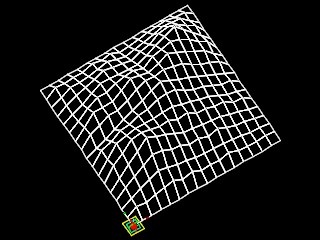
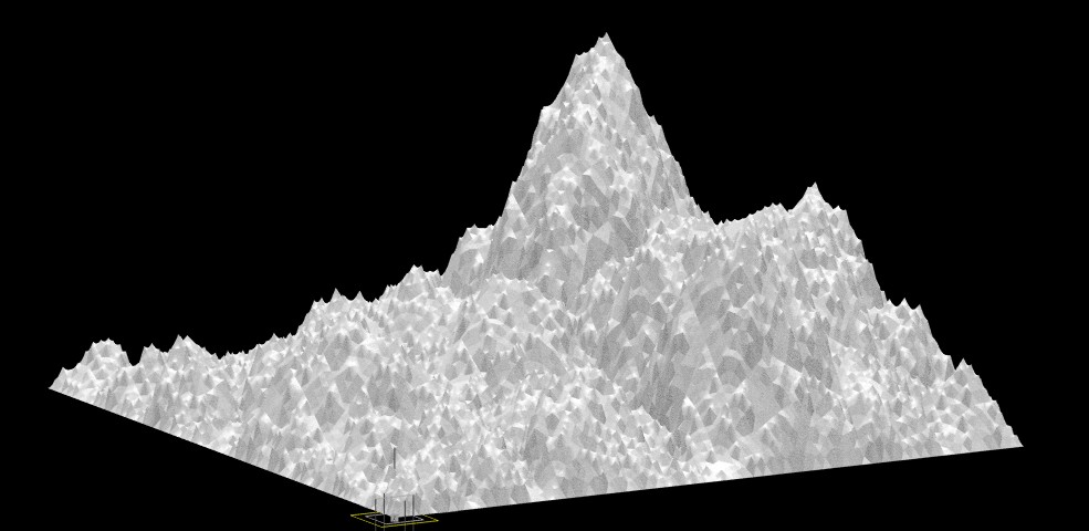
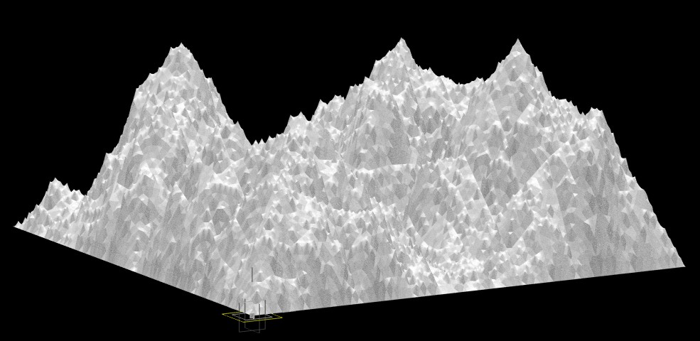
If the fractal mountain program is run for an increasing number of recursions (i.e., the value of recur is 6 or 7, then the peaks within the mountain become more numerous and dense. For the a following image, the assignment of the value recur = 7 is used in the function mountainGrid, and a simple texture map is applied to the resulting fractal pyramids. The image below is a close-up of the large mountain fractal which is formed. In practice, changing the roughness coeficient roughnessCoef from 0.6 to 0.5 does not produce remarkably noticeable differences. However, going to roughnessCoef 0.4 (not show) does result consistently in a smoother mountain surface. The mountains are also different due to a different set of random numbers used to generate each one.

Although the function makeGrid is written with a for loop, it is recursive in its approach towards the self-similar pyramid forms. Trying to write this procedure recursively would have been problematic due to performance related issues and memory management that is beyond the scope of this chapter.

fractal mountain for recur = 7 roughness coeficient = 0.6

fractal mountain for recur = 7 roughness coeficient = 0.5

Summary

Within this chapter, we have explored the use of recursive functions. A recursive function is one that calls itself in order to complete a task in which it is engaged. It typically ends when it encounters a grounding condition where the value of some variable reaches a limit (e.g., recur = 1). A recursive function continues to invoke itself when it encounters a recursive condition where the value of some variable has not yet reached a limit (e.g., recur > 1).

A recursive function was used to generate the rotating squares of the first example. The same graphic composition might alternatively have been created using an iterative program as we had seen in chapter 3. The recursive program style, however, seems to express most directly the self-similar nature of fractal graphics. That is, a program that calls itself is like a fractal that has parts that resemble its overall composition. Still, all of the recursive programs of this chapter might have been rewritten with even greater efficiency with the use of iterative loops. This is an exercise that could be explored by the reader using the iterative techniques described in chapter 3. Therefore, the advantage of developing the program recursively is not necessarily computational performance but rather clarity and conciseness of the code.

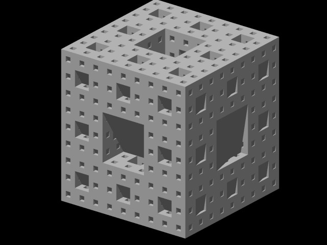
The fractal programs we have seen were very similar in their use of the variable recur to control the progression towards grounding condition. We have observed that that the recursive function drawrPyramid of the program that draws the fractal pyramids is similar in structure to the recursive function drawrtri of the program that draws the 2d fractal triangles. In turn, we have also observed that the iterative function mountainGrids similar in structure to the recursive function drawrPyramid of the script that draws the 3D pyramid fractal. A similar approach can be applied to recursively drawn cubes as in the assignment below and other such kinds of graphic compositions. However, in the next chapter we will also look at alternative approaches to generating fractal images where the property of self-similarity holds, but where the other means than a variable like recur drive the graphics construction process.

Assignment 8: Fractals and Final Exercise