WORKSHOP/SEMINAR
PARAMETRIC
RAPID PROTOTYPING: Chapter 8
For
Internal UVa. Use Only:
Draft: April 7, 2008
Copyright © 2008 by Earl Mark, University of Virginia, all
rights reserved.
Disclaimer |
Pre Fabrication Planning
This
chapter develops a few examples of pre-fabrication planning where a
surface is converted to a polygon grid, and, in turn, the polygon grid
is projected to a two-dimensional plan for cutting. The first example
is based upon a bspline surface developed by hand. The second example
is based upon a bspline surface that has been derived from a hyperbolic
parabolic surface developed as a graphics function . The specific
projection into a two dimension surface is done
using Generative Components functions, but the methods used are
generally applicable to the projective approaches available in most
other CAD systems.
The specific advantage of this parametric approach is that the
projection is modified in real time as a function according to
real-time changes to the projected surfaces.
Bpline
Surface
The
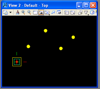
first example fabplanA.gct begins with placing four points by hand in the ground
plane.
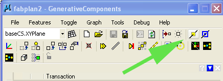
STEP 1: The Create Point icon highlighted the green arrow below can be used to place these points by hand.
The points should be placed roughly in the following manner.
STEP 2: The feature BSplineCurve is detetmined by the four points according to the ByPoles update metehod.
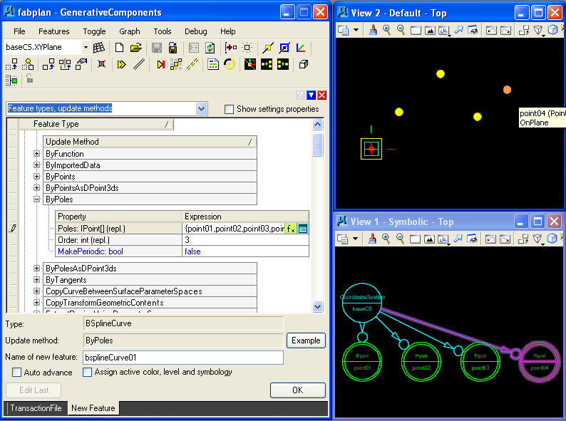
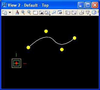
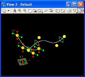
The resulting bspline curve appears as follows.
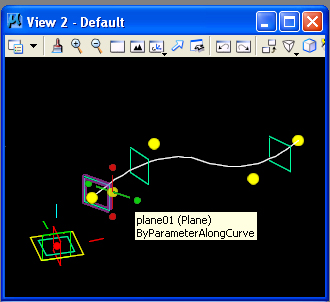
STEP 3: Three planes are placed along the bspline curve according to the ByDistanceAlongCurve update method, at the distances of 0.1, 0.5 and 0.9.
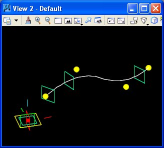
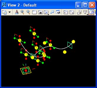
The three planes appear as follows.
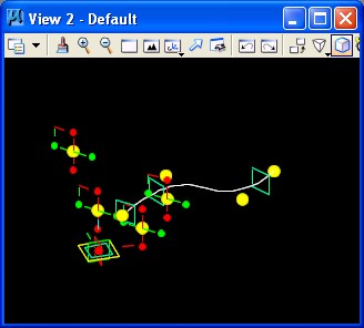
STEP 4: Again using the place point feature as in STEP 1, four
points are placed on the first of the three planes. Note that holding
the "ctrl" key down and
letting the mouse rest on any of the planes will convert the placement
of a point to its construction plane. The point itself is placed by
hitting the left-mouse button.
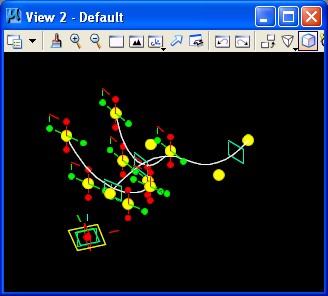
The result of placing ffour points on the first plane is as follows.
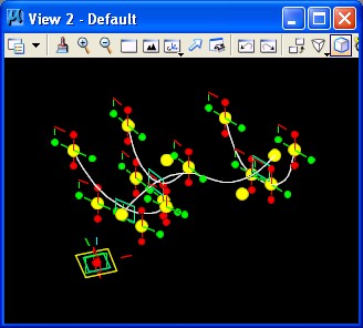
STEP 5: Using the method of STEP2, determine a BSplineCurve by the four points. The result of adding the BSplineCurve is as follows:
STEP 6: Again using the place point feature as in STEP 1, four points are placed on the second of the three planes.
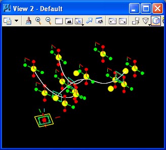
STEP 7: Again using the method of STEP2, determine a BSplineCurve on the second plane by the four points. The result of adding the BSplineCurve is as follows.
STEP 8: Further still using the place point feature as in STEP 1, four points are placed on the third of the three planes.
STEP 9: Again using
the method of STEP2, determine a BSplineCurve on the third plane by
the four points. The result of adding the BSplineCurve is as follows.
STEP 10: Create a BSplineSurface based upon the LoftCurves update method.
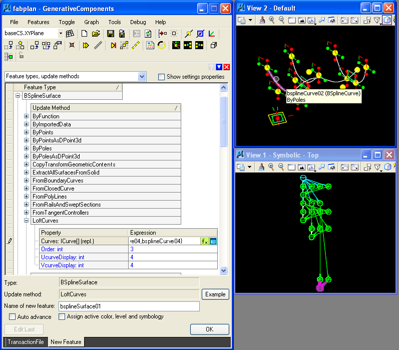
The result of adding the BSplineSurface is as follows.
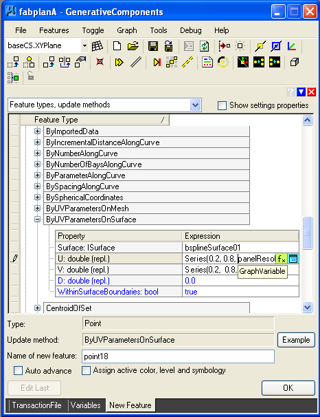
STEP 11: Create a Point along the BSplineSurface by the ByUVParametersOnSurface method.
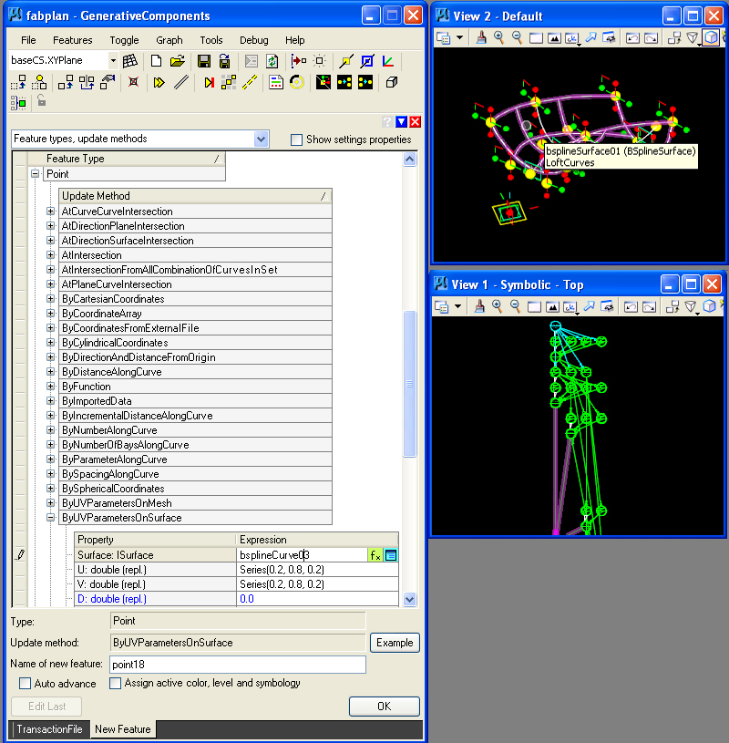
Note that U and V values for the point along the surface are entered as a Series. The Series(0.2, 0.8, 0.2) is a set of numbers beginning with minimum value of 0.2, and maximum value of 0.8, and an incremental value of 0.2. Thus, the series consists of the numbers 0.2, 0.4, 0.6, and 0.8. More generally, a Series(a, b, c) is a set of numbers with a minimum value of a, and maximum value of b, and incremental values of c. The resulting specification creates a set of four diagonal points with U, V values:
0.2,0.2
0.4, 0.4
0.6, 0.6
0,8, 0.8
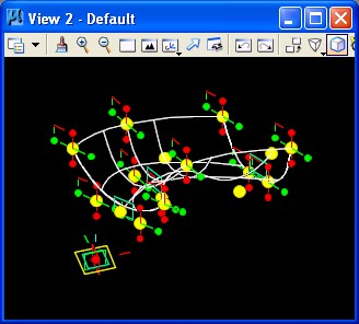
These are the points depicted on a diagonal from the lower left-hand corner to the upper right-hand corner of the surface below.
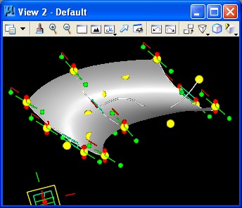
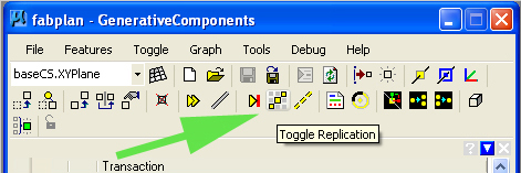
STEP 12: Using the Toggle Replication tool, these four diagonal points are reconstituted such that they form a grid of 16 spoints. The Toggle Replication tool selected off the main tool menu and then one of the four ponts is selected with the "ctrl" key to create the gird.
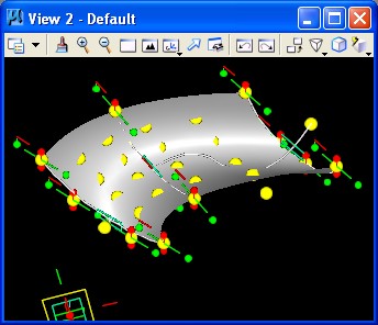
The sixteen U, V points are as follows.
0.2, 0.2
0.2, 0.4
0.2, 0.6
0.2, 0.8
0.4, 0.2
0.4, 0.4
0.4, 0.6
0.4, 0.8
0.6, 0.2
0.6, 0.4
0.6, 0.8
0.8, 0.2
0.8, 0.4
0.8, 0.6
0.8, 0.8
The replicated points now appear on the surface as depicted in the following image.
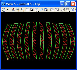
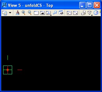
STEP 13: For
flattened layout of the point grid as a polygon, a new
CoordinateSystem feature is needs to be created using the AtModelOrigin method. Note that the text string "unfoldCS" is entered with quotation marks.
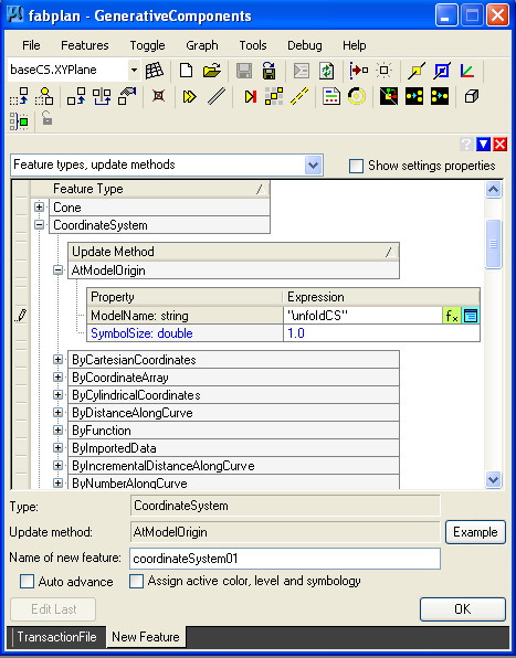 .
.
This results in the opening of a new view window number 5 depicting the new coordinate system.
STEP 14: A polygon is generated from the point grid of STEP 11 by means of the byPointGrid update method.
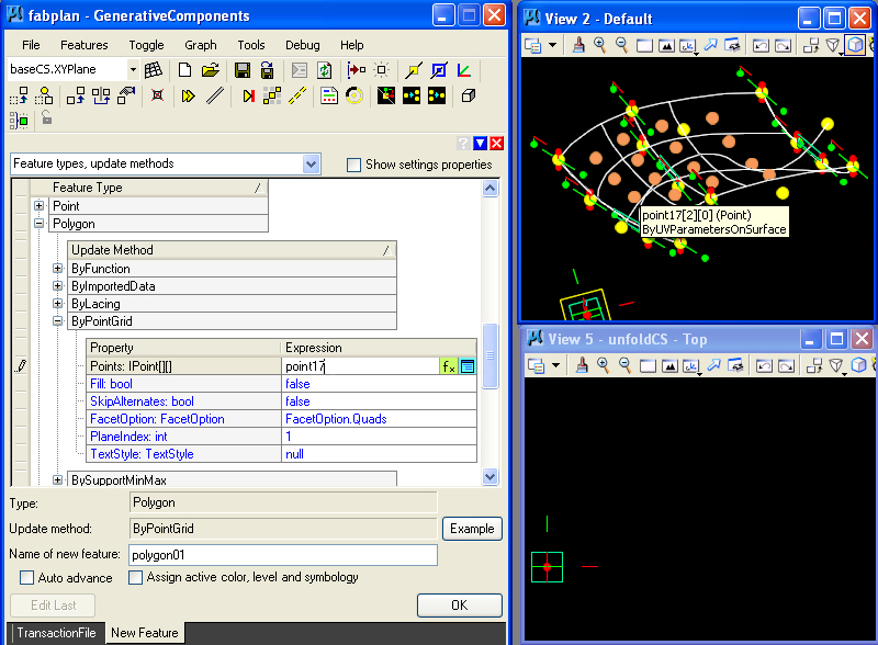
The polygon
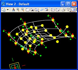
grid is created as depicted in the following view. This is the 16 point
grid depicted at the center of the BSplineSurface.
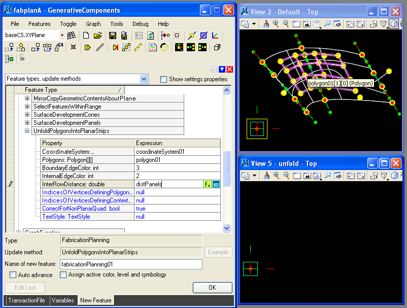
STEP 15: Finally, a FabricationPlanning feature is created by means of the UnfoldPolygonsIntoPlanarStrips
method. This feature is created with BoundaryEdgeColor 3, and
InternalEdgeColor 2, based upon the numerical color table for the
model. The InterRowDistance of 1 determines the spacing between
panels in the layout of the panels. The specification coordinateSystem01 relates to the new coordinate system determined by step 14.
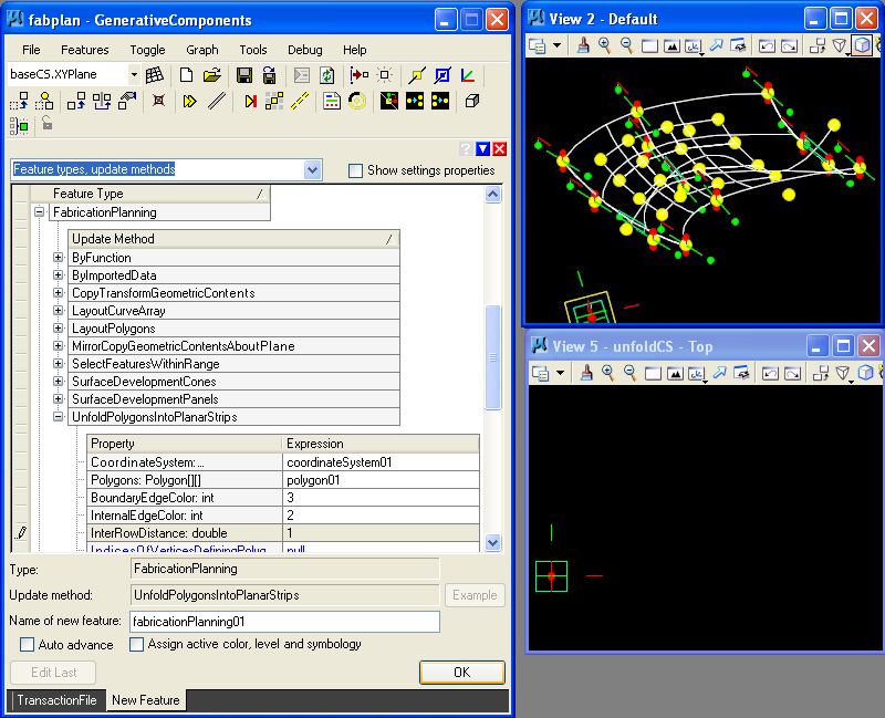
The resulting unfolded polygon is then depicted in View 5 as follows.
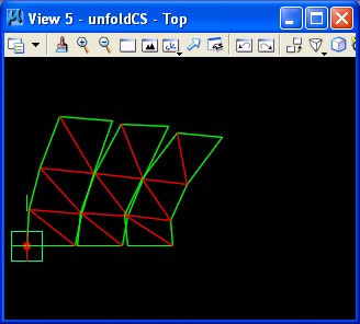
This unfolded panel can now be sent to the laser cutter or other fabrication device.
Bpline
Surface With Graphic Control Variables
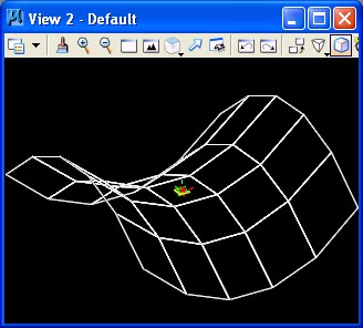
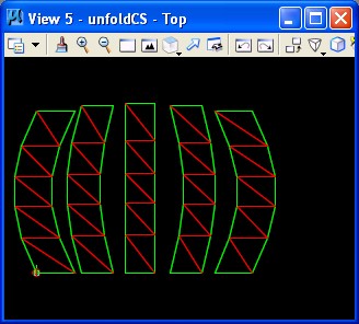
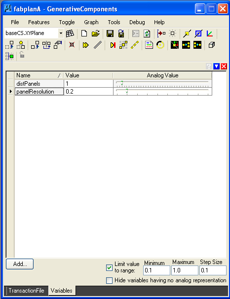
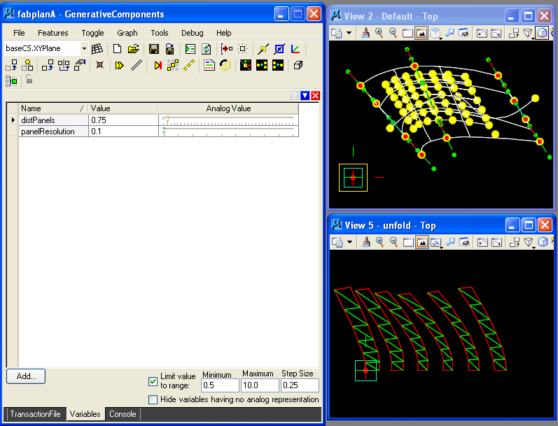
This
unfolded panel can be more directly maninpuated, as developed in fabplanB.gct, by creating two graphic
variables and parameterizing the size of the panels in STEP 11 above,
as well as parameterizing the distance between the panels in STEP 15
above. That is, repeating the entire process, we add a new first step.
NEW STEP 0: Create graphic variablesfor distancePanels and panelResolution, where panelResolution ranges from a minimum value of 0.1 to a maximum value 1.0 by step size 0.1, and distancePanels ranges from a minimum value of 0.25 to a maximum value 10.0 by step size 0.25.
NEW STEP 11: Former step 11 is now replaced with a new specification of series which is dependent upon panelResolution.
NEW STEP 15: The InterRowDistance of 1 from the previous STEP 15 determines the spacing between
panels in the layout of the panels. The graphic variable distPanels now allows this spacing to be more easily adjustable.
Here, for example, the graphic variables are adjusted to provide a
higher resolution of 0.1 and a new distance between panels of 0.5.
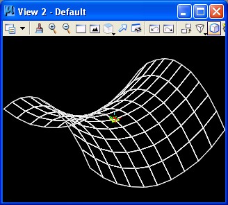
Hyperbolic Surface With Scripted Function
A hyperbolic parabolic surface, such as that depicted in Chapter 7, can
be unfolded using a combination of a function to derive a
BSplineSurface, and then by using the equivalen t of steps STEP 11
through STEP 15 above.
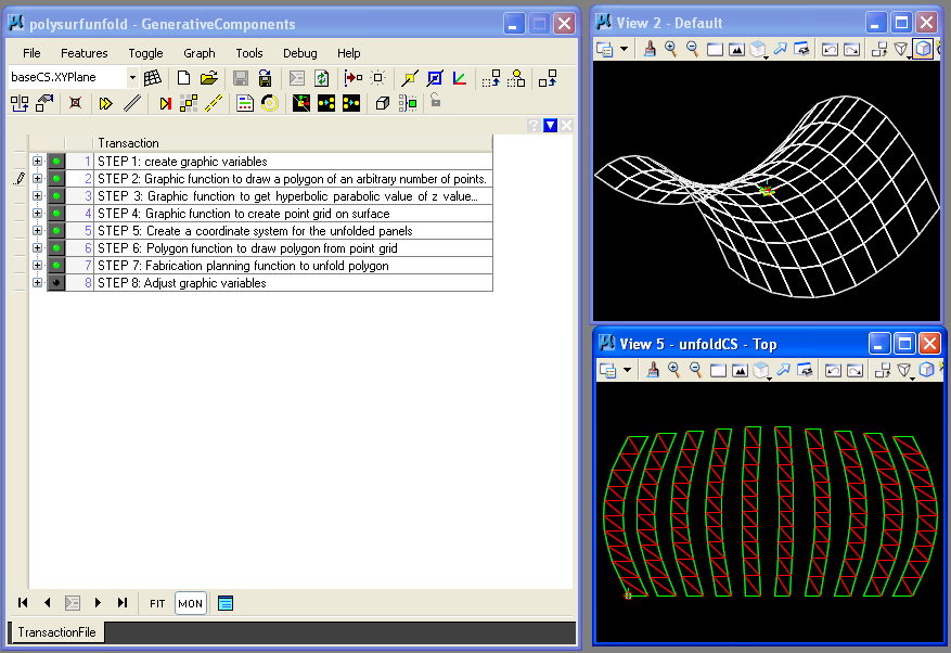
In the script polysurfunfold.gct we
control the resolution of the panels as well as the spacing between
them through the use of graphic variables. The primary work of the
generative
components transaction file is done in STEP 3 where we write a function
to create hyperbolic parabolic values of the surface, and in STEP 4
where
we write a function to generate a point grid on that surface and
replicate it. The remaining steps are handled with manual
methods. The graphics function for STEP 4 is reproduced in the text box
below.
The
graphics function is similar to that which was used to generate the
hyperbolic parabolic polygons of Chapter 7. However, here we are
generating a series of parallel PolyLines within the inner While loop.
The point pt1 increments along the y-axis according to the variable Resolution. The successive set of points are saved in the Point array polyPts. in the inner While loop.
while (yval <= MaxY) {
Point pt1 = new Point();
pt1.ByCartesianCoordinates(baseCS, xval, yval, zval);
pt1 = surfProc(pt1, Cscalar);
polyPts[i] = pt1;
i++;
yval = yval + Resolution;
}
The outer while loop draws each of the series of parallel PolyLines with the expression:
polyLines[ii] = drawPoly(polyPts);
Finally, these PolyLInes are lofted to create a BSPlineSurface with the expression:
hypSurf.LoftCurves(polyLines, 3);
From this point on, the balance of the work is handled in a similar manner to the preceding example of fabplanB.gct.
Note that variation on the parameters gives us a wide range of panelized altenrnatives:
By variation on the function of STEP 3, we can panelize the types of surface geometry reviewed in Chapter 7.