WORKSHOP/SEMINAR
PARAMETRIC RAPID PROTOTYPING: Chapter 5

Introducing Three-Dimensional Geometry and Polynomial Surfaces

This chapter lays out some basic concepts and examples of scripting  three dimensional surfaces. A foundation for construction of three dimensional geometry begins with Euclid's theorem which states that three points determine a plane. We first use three points to develop a construction plane, and then we apply construction planes to generating geometry.

The chapter also develops more completely the use of functions. The functions provide modularity to the programs, where the organizational breakdown of graphic composition is reflected in the organizational breakdown of how the code is structured. In effect, the code is a mirror of the geometry, reflecting its logic and providing a concise description that can be exploited for exercising variation.

In this chapter, we will also begin to use additional pre-defined object classes for creating drawing entities.

We are indebted to Descartes for our  present geometrical description of three-dimensional space. Descartes' development of Cartesian coordinates allowed problems in geometry to be reformulated into those in algebra (Ian Stewart,From Here to Infinity, Oxford University Press, 1996). We have already taken Descartes' important contribution for granted in the computer programs that rely upon two-dimensional coordinate geometry of the last chapters. We now move onto the vector algebra of three-dimensional space. We begin with simple rectangular polygons. We then use rectangular polygons to create surface elements.

Towards the end of this chapter, again using Cartesian coordinates, we work out one of Serlio's three-dimensional examples and then expand upon it. Note that Serlio (1475 - 1554) preceded Descartes (1596 - 1650) by approximately one century, and so that this translation of Serlio's geometry into Cartesian coordinates is according to techniques not available in his time.

Construction Planes:

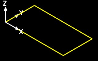
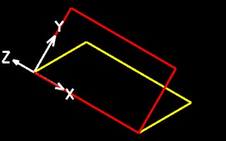
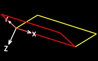
By convention, we can allow the three points to determine a specifically oriented Cartesian coordinate geometry where the first point determines the origin of a two-dimensional plane, the second point locates the x-axis and the third point gives the direction of the positive y-axis relative to the origin. The first figure below shows three such points identified in three-dimensional space. The second figure shows the positive x-axis and positive y-axis of a construction plane based on the initial three points. The third figure shows yet the direction of the positive z-axis relative to that construction plane.

3 Points Determine A Plane

The direction of positive z is determined according to the right-hand rule. The right-hand rule is a convention that is related to the use of the right hand. That is: (1) place the base of your right hand thumb at the origin such that the tip of the thumb points in the direction of positive-x and (2) orient your right-hand such that its index finger (next to the thumb ) is pointed in the direction of positive-y, then (3) your right-hand middle finger bends 90 degrees forward towards your palm to determine the direction of positive-z.

Any number of arbitrary construction planes may be defined by three points. In the example below, each construction plane contains the geometry of an intersecting circle and square.

A typical computer aided design system is based on the flexibility to describe three-dimensional geometry within any of these arbitrary construction planes. One such construction plane is designated as the Ground Construction Plane. It serves as the construction plane of basic reference and is typically co-planar with the ground plane of a three-dimensional model. Note that by convention, positive-y is pointed in the direction of North in the Ground Construction Plane, and by implication, negative-y is pointed in the direction of South, positive-x is pointed in the direction of East and negative-x is pointed in the direction of West. (Automated sun calculations are determined according to this convention, as can be adjusted to latitude, longitude and other factors).

The World Coordinate System and The Local Coordinate System

The World Coordinate System of a three-dimensional computer aided design model is typically synonymous with the coordinate system determined by the Ground Construction Plane. That is, three-dimensional points specified relative to the Ground Construction Plane are given directly in the World Coordinate System point values. For example, we might specify a 2 x 1 dimensioned vertical rectangle in the x-z plane with four corner points specified in World Coordinates of (0.0, 0.0, 0.0), (2.0, 0.0, 0.0), (2.0, 0.0, 1.0), (0.0, 0.0, 1.0). In all prior chapters, we have been creating geometry by default in the Ground Construction Plane.

A Local Coordinate System refers to the coordinate system of any currently active construction plane. It may refer to the coordinate system of any of the arbitrary construction planes illustrated above. Or, it may also refer to the coordinate system of the Ground Construction Plane if it is presently active. In all prior chapters, we have been creating geometry by default in the Local Coordinate System fully coincident with the Ground Construction Plane. In this chapter, we will also create geometry in alternative Local Coordinate Systems.

Three-Dimensional Specification Within A Computer Graphics Program

A three dimensional specification of geometry within a computer graphics procedure may be related to the x, y and z coordinate system of the Ground Construction Plane or of any of the arbitrary construction planes. For example, a line drawing in three-dimensional space may be specified in terms of its two end points (x1, y1, z1) and (x2, y2, and z2). Note that in chapter 2 we had predefined a data type Point that may hold the coordinate information of any given point

As we have already seen in earlier chapters, a point is declared in the GC script with the following expression:

Point curPoint = new Point();
curPoint.ByCartesianCoordinates(baseCS, x, y, z);

The first line above allocates memory for the point named curPoint. The second expression references baseCS. The World Coordinate System and the Ground Construction Plane are both the same baseCS construction plane. The second expression also constructs the point with  Cartesian coordinate values. That is, there is a field x declared as a double precision floating point number of the x-coordinate , a field y declared as a double precision floating point number of the y-coordinate, and a field z declared as a double precision floating point number of the z-coordinate of the three-dimensional point (review chapter 2 for more details).

Drawing A Polygon in the Local Coordinate System of the Ground Construction Plane: Trivial Case

We now write a number of GC scripts to draw polygons in any arbritrary local coordinate system.

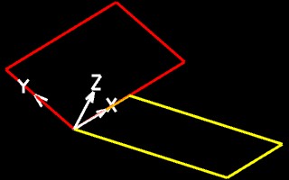
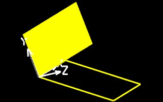
The GC script that is used below draws a Polygon in the Ground Construction Plane, baseCS. In this example program, the polygon is a simple 2 x 1 rectangle. When the procedure is modified further below, it draws a polygon in an alternative Local Coordinate System. Note that the white set of arrows is referred to as an Auxiliary Coordinate System icon and displays positive x, y, and z axis of the the currently active construction plane. The Auxiliary Coordinate System is synonymous with the currently active Local Coordinate System.

Yellow Rectangle in Ground Construction Plane

Red Rectangle in alternative Local Coordinate System

The polygon function in the box below contains a few new features. It includes a point array called pointList(), and it includes a technique for writing to a local coordinate system. We first write our procedure to draw the yellow rectangle in the left-hand figure above. We then modify the procedure to draw the tilted red rectangle in the right-hand figure above.

Within the procedure, the array called pointList is used to hold the values of the points that define the rectangle. The elements of the array are indexed according to a zero based scheme, where the first point is identified by pointList[0], the second point is identified by pointList[1], and in general, the nth point is identified by pointList[n - 1]. The x-component of the first point is identified by pointList[0].X, the y-component is identified bypointList([0].Y and the z-component is identified by pointList(0).Z. Or, more generally, the x-component of the point n is identified by pointList[n - 1].X, the y-component is identified by pointList[n - 1].Y, and the z-component is identified bypointList[n - 1]).Z. Arrays of points are a convenient shorthand for storing the values of a number of points. We can specify the size of the array with a statement such as Point pointList = {pt1, pt2, pt3}, where pt1, pt2 and pt3 are already established as Points. Or, we can initialize an array without determining its size with a statement such as  Point pointList = { };. According to the zero based index system, the statment Point pointList = { }; provides for an array that can handle up to any number of points, such as Points[0[, Points[1[, Points[2[ and Points[3[.

The declaration of the pointList array is sized dynamically when needed in the program. The dynamical declaration is unlike declarations we have seen before. We initialize the declaration of the array at one place and we determine the size of the array at another place. That is, we initially declare the pointListarray with the statement "Point pointList = { };" at the beginning of the polygon procedure. Later in the program, in the main body of the code, we specify the actual size of the array with the statements such as  "pointList[0] = pt1;" through "pointList[3] = pt4;". In different language, we would say that the size of the pointList array is allocated at runtime. The  "pointList[0] = pt1;" statement is a convenient technique for handling the allocation of array sizes dynamically when it varies according to the context in which the procedure is running, and we shall see why this may be useful in later examples.

The polygon function first sets up the location of the individual points in the default  Local Coordinate System which, as already noted, is also called baseCS and uses Cartesian coordinates. It then calls the graphics function drawPoly with the statement "drawPoly(pointList);". The graphics function drawPoly iis given the second box below and handles the actual creation of the polygon. Use of the baseCS constructor for each of the points in the polygon function means that the points are constructed relative to the World Coordinate System. In this default case,  the Auxiliary Coordinate System itself is equivalent to the World Coordinate System.

Within the graphics function drawPoly below, the points point1, point2,  point3 and point4 are submitted to the polygon constructor via the statment "arbitraryPolygon.ByVertices(pointList);" .

function () {

Drawing A Polygon in alternative Local Coordinate Systems: Non-Trivial Case

A modification to the polygon function changes the orientation of an Auxiliary Coordinate System to one that is tilted forward as represented by the ACS icon in the second of the two images above. That is, the change in the Auxiliary Coordinate System in turn causes the procedure to draw the red rectangle as depicted in the second image. The alternative polygon function relies on the definition of a new CoordinateSystem aux1CS. This coordinate system is created with the statement  "CoordinateSystem aux1CS = new CoordinateSystem(this);". 

The revised polygon function references aux1CS in the construction of pt1, pt2, pt3 and pt4.

You may wish to test the variations the construction plane occasioned by the following assignments of values to points orign, xaxisPt, and yxisPt, or experiment with other values..

Point origin = new Point(); origin.ByCartesianCoordinates(baseCS, 0.0, 0.0, 0.0); Point xaxisPt = new Point(); xaxisPt.ByCartesianCoordinates(baseCS, 1.0, 0.0, 0.0); Point yaxisPt = new Point(); yaxisPt.ByCartesianCoordinates(baseCS, 0.0, -1.0, 1.0);

Point origin = new Point(); origin.ByCartesianCoordinates(baseCS, 0.0, 0.0, 0.0); Point xaxisPt = new Point(); xaxisPt.ByCartesianCoordinates(baseCS, 0.0, 1.0, 0.0); Point yaxisPt = new Point(); yaxisPt.ByCartesianCoordinates(baseCS, -1.0, -1.0, 0.5);

Note that writing to an Auxiliary Coordinate System underscores the versatility of three-dimensional modeling techniques in computer aided design. In particular, an Auxiliary Coordinate System may help to simplify the description of drawing three-dimensional elements relative to other elements within a building or other three-dimensional object. For example, you might set the Auxiliary Coordinate System to be co-planar with the roof of a house, and then draw skylights and other elements relative to its geometry. Auxiliary Coordinate Systems are especially useful during development of a three-dimensional model where each command is input by the user manually through the available drawing tools one at a time rather than as facilitated by a computer graphics procedure.

We continue with using three-dimensional descriptions in the next example where we explore the creation of a closed polygon surface. For the sake of simplicity, however, we develop descriptions of surfaces with respect to the World Coordinate System only.  

Surface Descriptions

We first arrive at a surface description casually. The polygon function developed in the previous example created a closed three-dimensional rectangular surface. If we render the model appropriately, then it will reveal a closed rectangular surface rather than an open wireframe rectangle. In the illustration below, a rectangular surface element sits at an incline relative to the wireframe rectangle. The points used to determine the Auxiliary Coordinate System are the same as those used in the last example. Note that within a typical CAD system, the surface elements are rendered visible by using a shading tool. Within GC, the rendering tool is available under the utilities/render menu or directly from the viewing window. It is possible to choose from the menu a variety of rendering algorithms each with its own special effect. The rendering below is achieved with the filled hidden line algorithm. For a further discussion of rendering techniques, refer directly to the CAD system rendering tutorials.

Point origin = new Point(); origin.ByCartesianCoordinates(baseCS, 0.0, 0.0, 0.0); Point xaxisPt = new Point(); xaxisPt.ByCartesianCoordinates(baseCS, 0.0, 1.0, 0.0); Point yaxisPt = new Point(); yaxisPt.ByCartesianCoordinates(baseCS, -1.0, -1.0, 0.5);

A Polynomial Surface

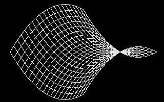
We have now established the basic foundation for developing a series of more advanced surface descriptions in three-dimensional space. In the examples below, polygons are described with reference to the World Coordinate System. This section picks out some polynomial expressions and the basic surfaces which they can produce. It is an eclectic collection derived from various textbook sources; however, there is consistency in how the basic surface elements are generated. In the examples given within this section, polynomial expressions are used to calculate the vertices of a number of simple four sided surface polygons. The four sided surface polygons are collectively arranged in three dimensional space so as to create larger surface areas. In the illustration below, we see a polygon wireframe description of a hyperbolic paraboloid shape on the left-hand side and its rendered surface description on the right-hand side [derived from Lord, The Mathematical Description of Shape and Form, John Wiley and Sons, 1984].

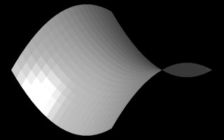Hyperbolic Paraboloid in wireframe and surface renderings

The x-coordinate and y-coordinate of the polygon vertices range over a set of values stepping in increments of 1 from -10 to +10. That is, we have -10 <= Point.x <= 10 and -10 <= Point.y <= 10. Note the regularity of this uniform x-coordinate and y-coordinate grid mesh is apparent when seen in the plan view as depicted below. However, the z-coordinate changes non-uniformly from vertex to vertex and accounts most directly for the curvature that is apparent in the views of the surfaces above.

Plan View of Hyperbolic Paraboloid in Wireframe and Surface Renderings

The full GC script  that generates the hyperbolic paraboloid surface will be given further below. First, however, we examine the logic of some of its parts. For each of the four sided polygons above, the z-coordinate value of each vertex is the function of its x-coordinate and y-coordinate values. The general mathematical expression used to calculate the z-coordinate of the vertices is:

where a, b and c are constants, z is the z-coordinate, x is the x-coordinate, and y is the y-coordinate value of a particular given polygon vertex in the figure above, and we use the symbol ^ to designate the exponentiation operator.  Note that to generate the specific surface above, a = b = 1.0, c = 0.1, -10 <= x < 10, and -10 <= y <= 10. Modification of the constants a, b and c change the relative curvature of the surface, but not its basic canonical shape.

The polynomial is equivalently expressed within a GC program more directly in terms of the z-coordinate each polygon vertexas:

In particular, examine the graphics function surfProc that takes a three dimensional Point and calculates its z coordinate Point.z based on the values of Point.x and Point.y e. The graphics function surfProc takes in a startPoint and scalar Cscalar and surfProc returns a new point named returnPoint  with the new z coordinate as indicated below.

Point function(Point startPoint, double Cscalar){
//Gets hybolic parabolic value of z from x and y of startPoint
Point returnPoint = new Point();
double a, b, xval, yval, zval;

//use standard polynomial equaltion to define value of "Z"
a = 1;
b = 1;

//note use of coeficients a & b not really needed in this case - same value if left out
zval = Cscalar  * ((Pow (startPoint.X, 2))/(a * a) - (Pow(startPoint.Y, 2))/(b*b));

//construct Return point with zval and original x-coordinate and y-coordinate values of startPoint
returnPoint.ByCartesianCoordinates(baseCS, startPoint.X, startPoint.Y, zval);

return returnPoint;

}

Sub procedure that calculates the z-coordinate of the hyperbolic paraboloid surface

To generate the surface, we need a way to organize every four adjacent vertices such that they form the individual polygons that constitute the overall surface. The following section of code contains two while loops that handle the work for some range of values in Point.X and Point.Y. In the outer loop, MinX < Point.x < MaxX, where MinX = - 10, MaxX = 10 and the x-coordinate values of the adjacent four vertices of a polygon are incremented by 1.0 during each iteration. Within the inner loop, MinY < Point.Y < MaxY, where MinY = -10, MaxY = 10, and the y-coordinate values of the adjacent four vertices of a polygon are incremented by 1.0 during each iteration. Also within the inner loop, we calculate the z-coordinate value of each polygon vertex point with a call to the sub procedure surfProc, and we draw each successive polygon with a call to the sub procedure drawPoly. Note that the use of variables MinX, MaxX, MinY and MaxY provide a convenient place in the code to control the range of x and y coordinate values over which the surface is generated.In other words, we might increase the surface area by setting MinX = -20, MaxX = 20, MinY = -20, MaxY = 20 or some other such assignment that would extend beyond the range of -10 to 10 for the x-coordinate and y-coordinate values.

 //Step through each face of surface
   while (xval < MaxX) {
      yval = MinY;
      yval2 = MinY + 1.0;

      while (yval < MaxY) {
  
         pt1.ByCartesianCoordinates(baseCS, xval, yval, zval);
         pt1 = SurfProc(pt1, Cscalar);
         pt2.ByCartesianCoordinates(baseCS, xval, yval2, zval);
         pt2 = SurfProc(pt2, Cscalar);
         pt3.ByCartesianCoordinates(baseCS, xval2, yval, zval);
         pt3 = SurfProc(pt3, Cscalar);
         pt4 = pt4.ByCartesianCoordinates(baseCS, xval2, yval2, zval);
         pt4 = SurfProc(pt4, Cscalar);
         drawPoly({pt1, pt3, pt4, pt2});
         yval = yval + 1.0;
         yval2 = yval2 + 1.0;
      }

      xval = xval + 1.0;
      xval2 = xval2 + 1.0;

   }

}

Fragment of sub procedure that processes four vertices of each polygon in 1 unit increments

The section of code we have generated thus far assumes that the x-coordinate and y-coordinate values of each point will increase in increments of 1.0, or, in other words, that each polygon is of a 1.0 x 1.0 dimension in the x - y plane. Alternatively, we could increase the resolution of the surface by reducing the increments to values of 0.5 so that each polygon is of a 0.5 x 0.5 dimension in the x - y plane.. Or more generally, we could use a variable called resolution so as to control the size of each polygon to a resolution x resolution dimension in the x - y plane as suggested in the following revised excerpt from the code.

Resolution = 1.0;

//Step through each face of surface
   while (xval < MaxX) {
      yval = MinY;
      yval2 = MinY + Resolution;

      while (yval < MaxY) {
  
         pt1.ByCartesianCoordinates(baseCS, xval, yval, zval);
         pt1 = SurfProc(pt1, Cscalar);
         pt2.ByCartesianCoordinates(baseCS, xval, yval2, zval);
         pt2 = SurfProc(pt2, Cscalar);
         pt3.ByCartesianCoordinates(baseCS, xval2, yval, zval);
         pt3 = SurfProc(pt3, Cscalar);
         pt4 = pt4.ByCartesianCoordinates(baseCS, xval2, yval2, zval);
         pt4 = SurfProc(pt4, Cscalar);
         drawPoly({pt1, pt3, pt4, pt2});
         yval = yval + Resolution;
         yval2 = yval2 + Resolution;
      }

      xval = xval + Resolution;
      xval2 = xval2 + Resolution;

   }

}

Fragment of sub procedure that processes four vertices of each polygon in increments of the variable resolution

If we set the value of our resolution to 0.5, then the resulting surfaces appear as developed in the illustrations below. The smaller resolution value of 0.5 effects a smoother approximation of the hyperbolic paraboloid surface.

Hyperbolic Paraboloid in Wireframe and Surface Renderings at resolution of 0.5

Lets return again to the parameters controlling the generation of the hyperbolic paraboloid surface.We refer in the expression below to the initial statement that determines the value of z. It can be observed directly and straightforwardly that the constant c controls the scale of z. That is, if we double the value of the constant c, then we would correspondingly double the scale of the z-coordinates of the resulting surfaces.

Within the graphics function procSurf, the constant c acts as a scalar. We give it name Cscalar to better associate the variable with its actual meaning. The z-coordinate value of  the vertice returnPoint of the hyperbolic parabolic surface is expressed within sub procedure SurfProc directly in terms of  the initial polygon vertex startPoint as:

a = 1;
b = 1;
zval = Cscalar  * ((Pow (startPoint.X, 2))/(a * a) - (Pow(startPoint.Y, 2))/(b*b));

//construct Return point with zval and original x-coordinate and y-coordinate values of startPoint
returnPoint.ByCartesianCoordinates(baseCS, startPoint.X, startPoint.Y, zval);

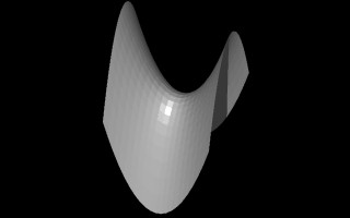
Within the following four illustrations, the value of Cscalar is increased in increments of 0.2. Each image has been re-scaled to fit the viewing frame (see the animation further below for relative scale). Reading the images from left to right and beginning with the first row, Cscalar values of 0.4, 0.6, 0.8 and 1.0 were used. Intuitively, it seems that the surface forms a kind of saddle. Since we form the hyperbolic paraboloid by squaring the values of x-coordinate and y-coordinate, we are not concerned with their positive or negative values, but rather with their distance from zero or, in other words, their absolute value. If the absolute value of the x-coordinate is high and the absolute value of y-coordinate is low, then the surface will rise up and the upper parts of the saddle are generated. If the absolute value of the x-coordinate is low and the absolute value of y-coordinate is high, then the surface will dip down and the lower parts of the saddle are generated. Middle range values for the x-coordinate and y-coordinate determine the middle levels of the saddle. Increasing the value of Cscalar accentuates the highs and lows of the surface form. Although not examined here for the sake of brevity, the impact of constants a and b might also be understood intuitively. If the absolute value of a < 1.0 and and the absolute value of b < 1.0, then it would have the impact of increasing the verticality of the surface as determined by the coordinates x and y respectively. Conversely, If the absolute value of a > 1.0 and and the absolute value of b> 1.0, then would have the impact of decreasing the verticality of the surface as determined by the coordinates x and y respectively.( Furthermore, since (Cscalar/2.0) is itself equal to a constant, we might substitute (Cscalar/2.0) with Cscalar thereby simplifying the equation slightly. However, if we retain the expression (Cscalar/2.0), then we find that setting the value of Cscalar to 0.1 often produce proportionately satisfying results, and the value of 0.1 seems to ground the expression in a useful way.)

We therefore re-express the fragment of code as:

a = 1;
b = 1;
zval = (Cscalar/2.0)  * ((Pow (startPoint.X, 2))/(a * a) - (Pow(startPoint.Y, 2))/(b*b));

//construct Return point with zval and original x-coordinate and y-coordinate values of startPoint
returnPoint.ByCartesianCoordinates(baseCS, startPoint.X, startPoint.Y, zval);

Cscalar values of 0.4, 0.6, 0.8 and 10.0.

The following animation depicts an increasing set of Cscalar values from 0.1 to 1.0. in increments of 1.0. Note that the surface changes in the z-axis only. Here, the scale of the images is maintained consistently so as to provide a relative size comparison of the different hyperbolic paraboloids.

Animation of Cscalar values of 0.1 to 1.0 in increments of 1.0

As we will see in later examples, it is useful to further isolate the Cscalar parameter in generating a number of other surface types. We also find that in many cases that negating the value of Cscalar inverts the resulting surface which is generated. Therefore, it becomes useful to redefine the sub-procedure SurfProc with Cscalar as an input variable that we can specify from the calling procedure. Adding Cscalar as an input variable to sub procedure surfProc is illustrated below.

Point function(Point startPoint, double Cscalar){
//Gets hybolic parabolic value of z from x and y of startPoint
Point returnPoint = new Point();
double a, b, xval, yval, zval;

//use standard polynomial equaltion to define value of "Z"
a = 1;
b = 1;

//note use of coeficients a & b not really needed in this case - same value if left out
zval = (Cscalar/2.0)  * ((Pow (startPoint.X, 2))/(a * a) - (Pow(startPoint.Y, 2))/(b*b));

//construct Return point with zval and original x-coordinate and y-coordinate values of startPoint
returnPoint.ByCartesianCoordinates(baseCS, startPoint.X, startPoint.Y, zval);

return returnPoint;

}

Sub procedure that calculates z-values of a hyperbolic paraboloid surface

Note that we have now identified a number of key variables that will play a significant role in the fully constructed GC script. The variable resolution controls the scale of the individual polygons of the procedure. Smaller values for resolution provide for smoother surfaces. The variable Cscalar controls the scale of the z-coordinate of the surface polygons, thereby providing a means to control its overall vertical size. The variables MinX, MaxX, MinY and MaxY determine the range of x and y coordinate values over which the surface is generated. The entire GC script polysurf.gct includes (1) a graphics function drawPoly to draw a polygon from an arbitrary number of points , (2) a graphics function surfProc to determine the z-coordinate value of each vertice, and a polygon function to iterate through the vertices of the grid.

(1) Graphics function drawPoly:

function (Point pointList){
//procedure to draw any closed polygon of unspecified number of points 

Polygon arbitraryPolygon = new Polygon(this);
                 arbitraryPolygon.ByVertices(pointList);

}

(2) Graphics function surfProc 

Point function(Point startPoint, double Cscalar){
//Gets hybolic parabolic value of z from x and y of startPoint
Point returnPoint = new Point();
double a, b, xval, yval, zval;

//use standard polynomial equaltion to define value of "Z"
a = 1;
b = 1;

//note use of coeficients a & b not really needed in this case - same value if left out
zval = (Cscalar/2.0)  * ((Pow (startPoint.X, 2))/(a * a) - (Pow(startPoint.Y, 2))/(b*b));

//construct Return point with zval and original x-coordinate and y-coordinate values of startPoint
returnPoint.ByCartesianCoordinates(baseCS, startPoint.X, startPoint.Y, zval);

return returnPoint;

}

(3) Polygon function;

Note that  more efficient method of drawing the polygon surface from lofted curves would reduce the amount of code used here, but the current function builds upon the conceptual approach of using simple polygons to build surfaces.

Procedure to draw a hyperbolic paraboloid surface

Other Surfaces Formed By Polygons

Note also that the modularity of this program permits the development of a number of other surface polygon procedures to be easily substituted for the hyperbolic parabolic script. These alternative surfaces may be generated by modifications only to the surfProc procedure.

A upside-down elliptical paraboloid [Clapham] type of surface is generated by the following substitute for the surfProc script. In particular, we have Point.z determined by the sum of the squares of Point.x and Point.y multiplied by Cscalar. Note that here we've not needed additional coeficients a and b as in the case of the hyperbolic parabolic script.

Point function(Point startPoint, double Cscalar){
//dome
Point returnPoint = new Point();
double zval;

//use standard polynomial equaltion to define value of "Z"
zval = (Cscalar / 2.0) * (Pow (startPoint.X, 2)) + Pow(startPoint.Y, 2));

//construct Return point with zval and original x-coordinate and y-coordinate values of startPoint
returnPoint.ByCartesianCoordinates(baseCS, startPoint.X, startPoint.Y, zval);

return returnPoint;

}

Sub procedure that calculates z-coordinate values of an elliptical paraboloid

If the absolute value of the x-coordinate is high and the absolute value of y-coordinate is high, then the surface will rise up and the upper parts of the dome are generated. This is true at the corners of the surface.  If the absolute value of the x-coordinate is low and the absolute value of y-coordinate is low, then the surface will dip down and the lower parts of the surface are generated. This is true in the middle of the surface. The surface below is generated for a value of Cscalar as 0.1.

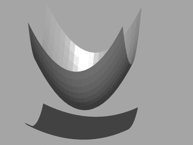An "upside-down" elliptical paraboloid with Cscalar set to 1.0

If we negate the value of Cscalar to -1.0, then the following surface is generated.

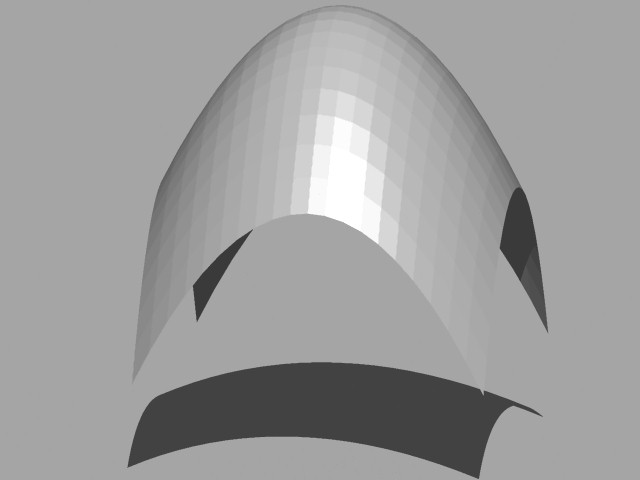An elliptical paraboloid with Scalar set to -1.0

This behavior of Cscalar when isolated appropriately also has similar reversal effects on most of the examples that follow. From their mathematical definitions, we arrive at the generation of these additional surfaces through modification of the surfProc procedure only. The scripts for graphics function drawPoly and the top level polygon function are not changed.. In each case, we are simply substituting another polynomial expression in parameters Point.x and Point.y to arrive at a value for Point.z.

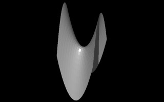
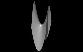
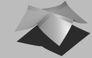
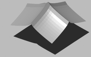
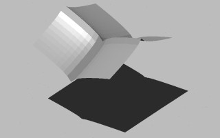
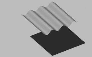
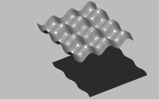
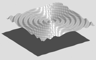
The script surfProc has been redefined for a set of case studies summarized in the following table. The script on the left corresponds to the surface generated on the right:

Point function(Point startPoint, double Cscalar){ //Gets simple saddle for z from x and y of startPoint Point returnPoint = new Point(); double zval; //use simple equation to define value of "Z" zval = Cscalar * startPoint.X * startPoint.Y; returnPoint.ByCartesianCoordinates(baseCS, startPoint.X, startPoint.Y, zval); return returnPoint; }
Point function(Point startPoint, double Cscalar){ // Gets chair-like saddle[derived from Lord] for z from x and y of startPoin // most effective for low values of Cscalar such as 0.01 Point returnPoint = new Point(); double zval; //use simple polynomial equation to define value of "Z" zval = Cscalar * (Pow(startPoint.X,2) + Pow(startPoint.Y,3)); returnPoint.ByCartesianCoordinates(baseCS, startPoint.X, startPoint.Y, zval); return returnPoint; }
Point function(Point startPoint, double Cscalar){ // Gets single ridge surf[derived from Lord] for z from x and y of startPoin // most effective for low values of Cscalar such as 0.01 Point returnPoint = new Point(); double zval; //use simple polynomial equation to define value of "Z" zval = Cscalar * (Pow(startPoint.X,2) - (Pow(Abs(startPoint.Y),0.667))); returnPoint.ByCartesianCoordinates(baseCS, startPoint.X, startPoint.Y, zval); return returnPoint; }
Point function(Point startPoint, double Cscalar){ // Gets high peak double ridge surf[derived from Lord] for z from x and y of startPoin // most effective for low values of Cscalar such as 0.5 Point returnPoint = new Point(); double zval; //use simple polynomial equation to define value of "Z" zval = Cscalar * -1 * Pow(Abs(startPoint.X * startPoint.Y),0.667); returnPoint.ByCartesianCoordinates(baseCS, startPoint.X, startPoint.Y, zval); return returnPoint; }
Point function(Point startPoint, double Cscalar){ // Gets high peak ridge surf with steep sloping sides[derived from Lord] for z from x and y of startPoin // most effective for low values of Cscalar such as 0.5 Point returnPoint = new Point(); double zval; //use simple polynomial equation to define value of "Z" zval = Cscalar * -1 * (Pow(Abs(startPoint.X), 0.6667) - Pow(Abs(startPoint.Y),0.667)); returnPoint.ByCartesianCoordinates(baseCS, startPoint.X, startPoint.Y, zval); return returnPoint; }
Point function(Point startPoint, double Cscalar){ // Gets dip and double ridge surface with steep sloping sides[derived from Lord] for z from x and y of startPoin // most effective for low values of Cscalar such as -0.1 (reverse up and down direction) Point returnPoint = new Point(); double zval; //use simple polynomial equation to define value of "Z" zval = Cscalar * -1 * Pow((Abs(startPoint.X * startPoint.Y)),0.667); returnPoint.ByCartesianCoordinates(baseCS, startPoint.X, startPoint.Y, zval); return returnPoint; }
Point function(Point startPoint, double Cscalar){ // Gets sin wave along y-axis for z from x and y of startPoin // Works well for Cscalar set to 1.0 with Resolution set to 0.5 Point returnPoint = new Point(); double zval; zval = Cscalar * Sin(Degrees(startPoint.Y)); returnPoint.ByCartesianCoordinates(baseCS, startPoint.X, startPoint.Y, zval); return returnPoint; }
Point function(Point startPoint, double Cscalar){ // Gets sin wave along x-axis and y-axis for z from x and y of startPoin // Works well for Cscalar set to 1.0 with Resolution set to 0.5 Point returnPoint = new Point(); double zval; zval = Cscalar * (Sin(Degrees(startPoint.X)) + Sin(Degrees(startPoint.Y))); returnPoint.ByCartesianCoordinates(baseCS, startPoint.X, startPoint.Y, zval); return returnPoint; }
Point function(Point startPoint, double Cscalar){ // Gets concentric wave values for z from x and y of startPoint // Works well for Cscalar set to 0.3 with Resolution set to 0.5 Point returnPoint = new Point(); double zval; double wavescl, dist; wavescl = 0.75; dist = Sqrt(Pow(startPoint.X,2) + Pow(startPoint.Y,2)); zval = Cscalar * Sin (Degrees((1.0 / wavescl) * dist)); returnPoint.ByCartesianCoordinates(baseCS, startPoint.X, startPoint.Y, zval); return returnPoint; }
Point function(Point startPoint, double Cscalar){ // Gets concentric wave with attenuation - discontinuous procedure values for z from x and y of startPoint // Works well for Cscalar set to 3.0 Point returnPoint = new Point(); double zval; double wavescl, attenfac, dist; wavescl = 0.75; dist = Sqrt(Pow(startPoint.X,2) + Pow(startPoint.Y,2)); if (Abs (dist) > 0.5) { attenfac = 2.0 / dist; } else { attenfac = 1.0; } zval = Cscalar * attenfac * Sin (Degrees((1.0 / wavescl) * dist)); returnPoint.ByCartesianCoordinates(baseCS, startPoint.X, startPoint.Y, zval); return returnPoint; }
Point function(Point startPoint, double Cscalar){ // Gets peak - discontinuous function values for z from x and y of startPoint [derived from procedure by Lord] // Works well for Cscalar set to -3.0 Point returnPoint = new Point(); double zval; if ((Pow(startPoint.X,2) + Pow(startPoint.Y,2)) >= 1) { zval = Cscalar * Log(Pow(startPoint.X,2) + Pow(startPoint.Y,2)); } else { zval = Cscalar * Log(1.0); } returnPoint.ByCartesianCoordinates(baseCS, startPoint.X, startPoint.Y, zval); return returnPoint; }

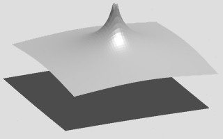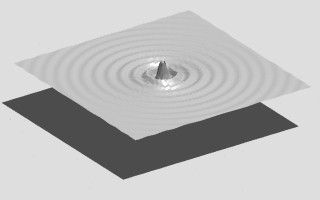
Note that the case of the concentric wave with attenuation in the example above involves the use of a a discontinuous function. That is, the variable dist is equal to the square root of the sum of the squares of point.x and point.y (i.e., dist = Sqrt(Pow(startPoint.X,2) + Pow(startPoint.Y,2)); ). If dist is equal to zero, then the expression attenfac = 2.0 / dist would involve division by zero. Therefore, for the sake of preserving the continuous shape of the wave, in all cases where dist < 0.5, we set atttenfac = 1.0. A similar use of a discontinuous function is used to control the shape of the peak in the next example, in this case to avoid calculating the log of 0.0.

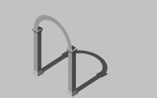
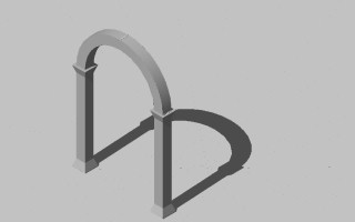
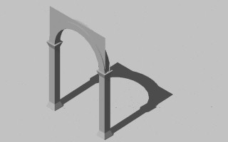
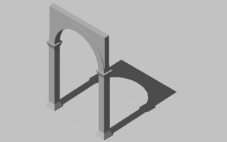
Serlio's Simplified Description of Columns, Arches, and A Recessed Square

A more complicated application of surfacing technique may be adapted to Serlio's didactic example of a recessed square sitting upon arches and supported by columns. He develops this description for the purpose of teaching perspective rendering with the "the arches drawn simply so as to accommodate their bases and capitals" [Hart]. Serlio was primarily concerned with a simplification of geometry so as to facilitate a drawing lesson in perspective. We may also find within it a way to understand the geometry of a recognizable composition of classical elements by breaking it down into a number of smaller drawing functions. The columns in Serlio's drawing lack detail in their depiction off base, shaft and capital, but retain the essential proportions of these parts. The arches in Serlio's example are simple roman arches. Serlio's description lends itself well to replication within a computer script serlioarch.gct. As in our earlier case studies, we rely greatly upon four sided polygons in a description. We also add a few new kinds of elements.

Views of Serlio's Column, Arch, and Recessed Square Composition (Axonometric, Plan and Perspective Views)

We begin our analysis of the composition by first approximating the perspective orientation as that described by Serlio in Book II, plate 43v with some shadow details added.

Here again we first examine the composition in its various parts before reviewing the computer graphics procedure as a whole. This code is necessarily complicated by two factors: (1) we are creating the above figure mainly with four sided polygon surfaces, which vary greatly in their geometry and spatial orientation, and (2) we interface with the somewhat idiosyncratic geometrical features of a scripting system. These complications are not untypical of programming a CAD system and so our approach to this example is generally applicable to other architectural case studies that consist of a number of distinct shapes.

Lets examine the columns first. Within the drawing above, note that each column might be described as a tall box with truncated pyramid boxes of a base and capital. To begin our description of the column we develop the graphics script below for a box. The box is centered at its base at centrPt. It has dimensions for bottom box length bLen, bottom box width bWid, and also top box length tLen, top box width tWid, and box height vertDim. These dimensions are in turn used to calculate a rectangle consisting four points pointsBot() at the bottom of the box and four points pointsTop() at the top of the box. Finally, the points pointsBot() and pointstop() determine the vertices of the six polygons that form the faces of the box. Each of the polygons is then drawn separately.

Note that the specification of the box permits the top face and lower face to have different dimensions. Therefore, the base of the column may be represented by a truncated pyramid type box with the bottom polygon face larger than the top polygon face. Conversely, the top of the column is represented by an upside-down truncated pyramid type box with the bottom polygon face smaller than the top polygon face.

function(Point centerPt, double bLen, double bWid, double tLen, double tWid, double vertDim){
//Make a box from six four sided polygons 
Point pointsBot = {};
Point pointsTop = {};
double zval;

// Calculate corner points of base rectangle
   pointsBot = calcRect(centerPt, bLen, bWid);

// Calculate corner points of top rectangle
   pointsTop = calcRect(centerPt, tLen, tWid);
   
   pointsTop[0].ByCartesianCoordinates(baseCS, pointsTop[0].X, pointsTop[0].Y, centerPt.Z + vertDim);
   pointsTop[1].ByCartesianCoordinates(baseCS, pointsTop[1].X, pointsTop[1].Y, centerPt.Z + vertDim);
   pointsTop[2].ByCartesianCoordinates(baseCS, pointsTop[2].X, pointsTop[2].Y, centerPt.Z + vertDim);
   pointsTop[3].ByCartesianCoordinates(baseCS, pointsTop[3].X, pointsTop[3].Y, centerPt.Z + vertDim);

// Draw Polygons for each side of box
   drawPoly(pointsBot[0], pointsBot[1], pointsBot[2], pointsBot[3]);
   drawPoly(pointsBot[0], pointsBot[1], pointsTop[1], pointsTop[0]);
   drawPoly(pointsBot[1], pointsBot[2], pointsTop[2], pointsTop[1]);
   drawPoly(pointsBot[2], pointsBot[3], pointsTop[3], pointsTop[2]);
   drawPoly(pointsBot[3], pointsBot[0], pointsTop[0], pointsTop[3]);
   drawPoly(pointsTop[0], pointsTop[1], pointsTop[2], pointsTop[3]);

}

The graphics function makeBox relies upon the graphic function calcRect to determine the actual points. This delegation of some of the work of the function to another function simpliefies the logi of makeBox. The additional logic of the function calcRect can be deferred to a lower level process and alleviates some complexity. The graphics function calcRect is as follows:

function(Point centerPt, double bLen, double bWid, double tLen, double tWid, double vertDim){
//Make a box from six four sided polygons 
Point pointsBot = {};
Point pointsTop = {};
double zval;

// Calculate corner points of base rectangle
   pointsBot = calcRect(centerPt, bLen, bWid);

// Calculate corner points of top rectangle
   pointsTop = calcRect(centerPt, tLen, tWid);
   
   pointsTop[0].ByCartesianCoordinates(baseCS, pointsTop[0].X, pointsTop[0].Y, centerPt.Z + vertDim);
   pointsTop[1].ByCartesianCoordinates(baseCS, pointsTop[1].X, pointsTop[1].Y, centerPt.Z + vertDim);
   pointsTop[2].ByCartesianCoordinates(baseCS, pointsTop[2].X, pointsTop[2].Y, centerPt.Z + vertDim);
   pointsTop[3].ByCartesianCoordinates(baseCS, pointsTop[3].X, pointsTop[3].Y, centerPt.Z + vertDim);

// Draw Polygons for each side of box
   drawPoly(pointsBot[0], pointsBot[1], pointsBot[2], pointsBot[3]);
   drawPoly(pointsBot[0], pointsBot[1], pointsTop[1], pointsTop[0]);
   drawPoly(pointsBot[1], pointsBot[2], pointsTop[2], pointsTop[1]);
   drawPoly(pointsBot[2], pointsBot[3], pointsTop[3], pointsTop[2]);
   drawPoly(pointsBot[3], pointsBot[0], pointsTop[0], pointsTop[3]);
   drawPoly(pointsTop[0], pointsTop[1], pointsTop[2], pointsTop[3]);

}

Polygon function(Point Point1, Point Point2, Point Point3, Point Point4){
//Draws  polygon of four points
Polygon returnPolygon = new Polygon(this);
returnPolygon.ByVertices({Point1, Point2, Point3, Point4});

return returnPolygon;
}

The graphics function makeBox does much of the work of creating the Serlio composition. When appropriate dimensions are applied, we are able to create boxes for all the forms of his composition with the exception of (1) the rectangles at the base, and (2) the arches and the walls directly above the arches. The rectangles of the base are straightforward and similar to the simple polygons we have created before. The explanation for them will be left to the code itself. However, in order to create the arches and the walls above the arches, a new technique is introduced in the code.

Generate arch profile and project arch [top row], generate wall above arch and project wall [ bottom row] (columns shown for reference)

The graphics function drawArch first traces out the profile of the arch in elevation (see above illustration). The geometry of the arch is calculated straightforwardly with respect to its center point centerPt and radius archRadius, and also the distance between its introdos (inside arc) and extrados (outside arc) given as colBaseDim. As indicated in the graphics function, the extrados is drawn first, then the left-hand line which connects the extrados to the introdos, then the introdos, and then finally the right-hand line that connects the introdos to the extrados (see top left image in above table).Note that colBaseDim is also the length of the side of the square plan of the column . This is important since the base of the arch, the distance between its intrados and the extrados, is this same dimension and therefore fits exactly on top of the square of the column.)

In order to create an arc, we use the arguements startPoint, PointOnRadius, and endPoint define the beginning point, a point on the arc, and the end point of the arc.

Once having created the lines and arcs, we place them inside a composite arc referred to as compositeCurve. The compositeCurve is one that can can be formed from several geometrical elements, including the intrados, extrados and lines of the arch. The geoemtric elements held inside the compositeCurve are linked are constructedn and linked together  with the expression "compositeCurve.CompositeCurves({extradosArc,arcLeftLine, intradosArc, arcRghtLine});".

 This surface is then copied to the parallel side of the arch with the construction of a new projecteed complex arc referred to as  compositeCurveP.  The statement "compositeCurveP.CompositeCurves({extradosArcP,arcLeftLineP, intradosArcP, arcRghtLineP});" creates the second compositeCurve from copied elements of the first composite curve. The means of creating this curve requires that copies of each of the extradosArc, arcLeftLine, intradosArc, arcRghtLine are copied to correponding new gemetrical elements extradosArcP,arcLeftLineP, intradosArcP, arcRghtLineP. 

// Create a projected arch face
    Point copyTo = new Point();
    xval = vector.X;
    yval = vector.Y;
    zval = vector.Z;
    copyTo.ByCartesianCoordinates(baseCS, xval, yval, zval, centerPt);
    extradosArcP.CopyTransformGeometricContents(extradosArc, centerPt, copyTo);
    intradosArcP.CopyTransformGeometricContents(intradosArc, centerPt, copyTo);
    arcLeftLineP.CopyTransformGeometricContents(arcLeftLine, centerPt, copyTo);
    arcRghtLineP.CopyTransformGeometricContents(arcRghtLine, centerPt, copyTo);
    compositeCurveP.CompositeCurves({extradosArcP,arcLeftLineP, intradosArcP, arcRghtLineP});

Once the arch profile has been created for the two vertical surfaces of the arch, it is projected horizontally using the sub procedure projCurve2 (see top right image in above table). To understand how projCurve2 works in more detail, first review the code in the second box below, and then read the text that follows. The wall above the arch is created in a similar way of drawing its profile and then projecting it horizontally (see bottom row of images in the above table).

function(Point centerPt, double archRadius, double colBaseDim){
// Draw an arch
   Point startPoint = new Point();
   Point endPoint = new Point(); 
   Point pointOnRadius = new Point();
   Point vector = new Point();
   double xval, yval, zval;
   Arc extradosArc = new Arc();
   Arc intradosArc = new Arc();
   Arc extradosArcP = new Arc();
   Arc intradosArcP = new Arc();
   PolyLine arcLeftLine = new PolyLine();
   PolyLine arcRghtLine = new PolyLine();
   PolyLine arcLeftLineP = new PolyLine();
   PolyLine arcRghtLineP = new PolyLine();
   Curve compositeCurve = new Curve(this);
   Curve compositeCurveP = new Curve(this);

// Draw extrados of arch 
   xval = centerPt.X + archRadius;
   yval = centerPt.Y - (0.5 * colBaseDim);
   zval = centerPt.Z;
   startPoint.ByCartesianCoordinates(baseCS, xval, yval, zval );
   xval = centerPt.X;
   yval = centerPt.Y - (0.5 * colBaseDim);
   zval = centerPt.Z + archRadius;
   pointOnRadius.ByCartesianCoordinates(baseCS, xval, yval, zval );
   xval = centerPt.X - archRadius;
   yval = centerPt.Y - (0.5 * colBaseDim);
   zval = centerPt.Z;
   endPoint.ByCartesianCoordinates(baseCS, xval, yval, zval);
   extradosArc.ByPointsOnCurve(startPoint, pointOnRadius, endPoint);

// Draw left-hand line at base of arch
   xval = endPoint.X;
   yval = startPoint.Y;
   zval = startPoint.Z;
   startPoint.ByCartesianCoordinates(baseCS, xval, yval, zval);
   xval = endPoint.X + colBaseDim;
   yval = endPoint.Y;
   zval = endPoint.Z;
   endPoint.ByCartesianCoordinates(baseCS, xval, yval, zval );
   arcLeftLine.ByVertices({startPoint, endPoint});

// Draw intrados arch
   xval = endPoint.X;
   yval = startPoint.Y;
   zval = startPoint.Z;
   startPoint.ByCartesianCoordinates(baseCS, xval, yval, zval);
   xval = centerPt.X + (archRadius - colBaseDim);
   yval = endPoint.Y;
   zval = endPoint.Z;
   endPoint.ByCartesianCoordinates(baseCS, xval, yval, zval );
   xval = pointOnRadius.X;
   yval = pointOnRadius.Y;
   zval = pointOnRadius.Z - colBaseDim;
   pointOnRadius.ByCartesianCoordinates(baseCS, xval, yval, zval);
   intradosArc.ByPointsOnCurve(startPoint, pointOnRadius, endPoint);

// Draw right-hand line at base of arch
   xval = endPoint.X;
   yval = startPoint.Y;
   zval = startPoint.Z;
   startPoint.ByCartesianCoordinates(baseCS, xval, yval, zval );
   xval = endPoint.X + colBaseDim;
   yval = endPoint.Y;
   zval = endPoint.Z;
   endPoint.ByCartesianCoordinates(baseCS, xval, yval, zval );
   arcRghtLine.ByVertices({startPoint, endPoint});

// Link graphic elements together
    compositeCurve.CompositeCurves({extradosArc,arcLeftLine, intradosArc, arcRghtLine});
    
// Project arch according to plan thickness (colBaseDim)
    xval = 0.0;
    yval = colBaseDim;
    zval = 0.0;
    vector.ByCartesianCoordinates(baseCS, xval, yval, zval);
    
// Create a projected arch face
    Point copyTo = new Point();
    xval = vector.X;
    yval = vector.Y;
    zval = vector.Z;
    copyTo.ByCartesianCoordinates(baseCS, xval, yval, zval, centerPt);
    extradosArcP.CopyTransformGeometricContents(extradosArc, centerPt, copyTo);
    intradosArcP.CopyTransformGeometricContents(intradosArc, centerPt, copyTo);
    arcLeftLineP.CopyTransformGeometricContents(arcLeftLine, centerPt, copyTo);
    arcRghtLineP.CopyTransformGeometricContents(arcRghtLine, centerPt, copyTo);
    compositeCurveP.CompositeCurves({extradosArcP,arcLeftLineP, intradosArcP, arcRghtLineP});
    
// Create extruded portion of arch
    projCurve2(compositeCurve, vector);
}

function (Curve startCurve, Point vector) {
//project a polygon
Point startPoint = new Point();
Point endPoint = new Point();
Curve endCurve = new Curve();
double xval, yval, zval;
Point startPts = {};
Point projPts = {};

//Create points at ends of projection Vector away from element area
   xval = 0.0;
   yval = 0.0;
   zval = 0.0;
   startPoint.ByCartesianCoordinates(baseCS, xval, yval, zval);
   endPoint.ByCartesianCoordinates(baseCS, vector.X, vector.Y, vector.Z, startPoint);

//Create projected curve
  endCurve.CopyTransformGeometricContents(startCurve, startPoint, endPoint);
 

// Project the entity 
   BSplineSurface projSurf = new BSplineSurface(this);
   projSurf.LoftCurves({startCurve, endCurve});
    
}

Sub procedures to draw an arch profile and project it horizontally

The sub procedure projArc projects and arc according to the three-dimensional vector Vector. The first step within the function is to determine the start and end point of the vector : 

startPoint.ByCartesianCoordinates(baseCS, xval, yval, zval);
endPoint.ByCartesianCoordinates(baseCS, vector.X, vector.Y, vector.Z, startPoint);

The arch profile startCurve is copied and projected with the construction of a new endCurve according to the start and end points of the vector;

  endCurve.CopyTransformGeometricContents(startCurve, startPoint, endPoint);

The script then creates a suface on the projected curve with the statement:

BSplineSurface endCurveS = new BSplineSurface(this);
 endCurveS.FromClosedCurve(endCurve); 

 Next we take the original curve startCurve and the new curve endCurve and loft a new bspline surface inbetween them with the statements:

   BSplineSurface projSurf = new BSplineSurface(this);
   projSurf.LoftCurves({startCurve, endCurve});

 A seperate function projCurve2 is also included in the script to handle less complex cases where a simpler projection is all that is needed. In this later script, the projected curves isn not scripted.

The remaining functions to create the Serlio composition are based on the three techniques that we have now reviewed:

1. the creation of various kinds of boxes for the columns and beams;
2. the creation of simple rectangles for the base;
3. the projection of profiles for the arch and the wall above arch.

The graphic functions needed to complete Serlio's composition follow the same logic that we have seen in the graphics functions already review for this geometrical construction. All the specialized functions handle some  particular calculation of the geometry, and the location and specific dimensions of  architectural elements. Thhese specific calculations are commented on directly in the code. Some while loops are incorporated to handle repetitions of columns, arches, etc.. Thus, the entire set of functions appears now in the box below and is provided with comment lines in the code itself that explain its various parts. Note that these graphic functions appear below in the same order as in the GC script iteself given that there's a dependency of later procedures on the ones that they call upon and therefore need to be defined earlier. All but the final script are graphics functions. The final function is a polygon function that initiates and controls the entire process developed by the collected set of functions. 

    serlioArches(numRows, numCols, numLevels)

The polygon function  serlioArches takes three arguments numRows, numCols, and numLevels). These three arguements can also be controlled as graphic variable to drive the entire script, thus allowing for a variable number of arches controlled parametrically.

Complete procedure to draw Serlio's recessed square sitting upon arches and supported by columns

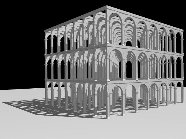
Finally, note that the sub main procedure of the code contains a number of key variables that control the dimensions and level of repetition in the composition. If NumRows = 3 and NumCols = 3 then we get a 3 x 3 array of columns, with each pair of columns supporting an arch above it. Furthermore, the variable BaseColDim is key to the entire scale of the composition. The scale can be doubled if we set BaseColDim = 2. Furthermore, we can begin to create several vertical levels of the composition if we set NumLevels = 3. Experimentation with the values to these variables will quickly yield a great range of possible repetitions of Serlio's initial composition. The image below represents one such variation where NumCols = 8, NumRows = 8 and NumLevels = 3. These variables can be further set aside as input arguments to the polygon function to create the series of arches, and parametrically be used to regenerate the composition. 

Summary

Within this chapter we have developed a few basic techniques for representing three-dimensional surfaces . The principal building block of these surface elements has been a four sided polygon. Initially we described how four sided polygons might be given any orientation in three-dimensional space as facilitated by the use of Local Coordinate Systems. We described how the lines within a four side polygon might be linked together to create a surface. We examined how such four side polygons could be arrayed together so as to create various kinds of polynomial and other surfaces. In our final example, we created a particular Serlio composition from four sided polygons that created boxes and also projected surface elements.

Our examples also demonstrates the power of encapsulating the basic parameters of a particular architectural composition within a few variables. In the case of polynomial related surfaces, we were able to succinctly describe the range of the surface (i.e., the variables MinX, MinY, MaxX, MaxY), the scale of its curvature (i.e., the variable Cscalar) and the resolution of its curvature (i.e., the variable resolution). In the case of Serlio's composition, we were able to control the basic scale (i.e., the variable colBaseDim), and the degree of repetition of the basic elements (e.g., the variables numCols, numRows and numLevels).

The capturing of an architectural composition into a few basic parameters harnesses the power of the computer to rmost directly assert the geometrical order of a design the variations possible. This kind of relation between code and architectural geometry always runs the risk of oversimplification. For example, our last procedure would need to be modified in order to incorporate scale and orientation changes for Serlio's composition. This kind of is adjustment is well within the concepts we have discussed and might be handled by modifying the code for Serio_Arccade.. More reflectively, however, we begin to assess here the computability of certain architectural forms, make educated assumptions about what is admitted within the main body of computer graphics procedure as central to an architectural composition, and what might be treated on an exceptional basis. This approach to geometrical modeling begins to address the real difficulty and interest of architecture, where the order of the whole composition is not easily described within one comprehensive prcedure description. Yet, we now have arrived at some general techniques difficult to do precisely by hand because of the precision of the calculations required. The hypbolic parabolic surface illustrated above is perhaps a best example of this. These methods will grow in sophistication as we capture the order of some additional architectural forms in fractals and solid models in the chapters that follow.

Assignment 6: Polynomial surfaces - Graphics to Physical Prototyping.